The display settings determine how the extracted elements, faces, and annotations (labels, coordinate system axes) will be displayed. Lighting and transformation settings are also part of the display settings.
In the graphical user interface, the display settings are
located on the Display page of the
NPart editor.
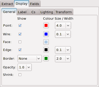
The display settings located on the first sub-page of the
NPart editor are the most commonly used
ones.
These settings determine if and how points and nodes, wire (line) elements, faces, and face edges are displayed. There are the following attributes:
-
show: If points, wire (line) elements, faces, or edges should be displayed. By default, points, wire elements, and faces are displayed, but no edges.To enable the display of edges in the graphical user interface, activate the corresponding check box. From the Python environment (assuming that "p" references the
NPartobject):p.edge.show = True
-
colour: The default colour. This colour is used when colouring by field values is inactive (default). To change these colours in the graphical user interface, click on the button displaying the colour. A dialog window appears, allowing to select a new colour. The colour can be entered as HSV- or RGB-values. In the Python environment, the "colour" property accepts RGB-values and the colour names defined by the X Consortium (like black, white, yellow, DarkSeaGreen, CornflowerBlue etc.). The RGB-values are integers between 0 and 255. Thus,p.point.colour = 'red'
and
p.point.colour = [255, 0, 0]
are identical.
-
sizeorwidth: The size (in pixels) for points, and the width (also in pixels) for wire elements and edges. The default width of 0.1 for wire elements and edges actually means 1 pixel width for OpenGL display, but in PostScript and PDF output, this will output hair lines.The following example makes wire elements 2 pixels wide:
p.wire.width = 2
The border of an NPart can be displayed
too; this is useful for meshes where the display of edges would give
a too fine pattern. The border can be displayed according to the
following criteria:
-
boundary: Borders will be drawn at 2D elements having no neighbours and at 3D elements making an edge or a corner. -
branch: Borders will be drawn between neighbouring elements belonging to different branches. -
group: Borders will be drawn between neighbouring elements having different element group codes. -
panel: Borders will be drawn between neighbouring elements having different element panel codes. -
sfvbc: Borders will be drawn between neighbouring elements having different element sfvbc codes (boundary conditions for NSMB flow solver models).
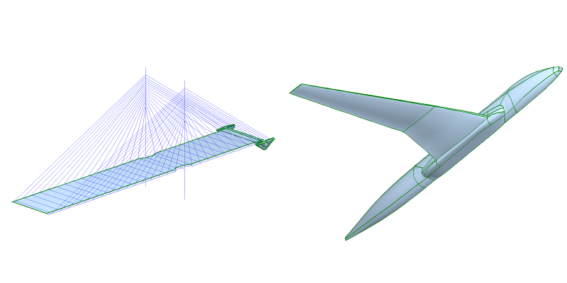
The following figure displays on the left side the bridge model with the boundary; on the right side, a wing-body configuration is displayed with borders on the branches (structured blocks).
These criteria can be combined. In the graphical user
interface, a drop-down combo box allows for activation of a
combination of these criteria. In the Python environment, the
border.show property is a comma-separated string.
For instance,
p.border.show = 'boundary,branch'
activates the boundary and
branch criteria.
The colour and width of the borders can be set in the same fashion as described in the previous section for the display of wire elements and edges. By default, borders are displayed 2 pixels wide and in a dark green.
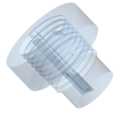
By default, an NPart is opaque. In some
cases it might be useful to allow for a certain amount of
transparency. This is achieved with the "opacity" property which
ranges from 0.1 (almost transparent) to 1.0 (fully opaque) in steps
of 0.1.
p.opacity = 0.3
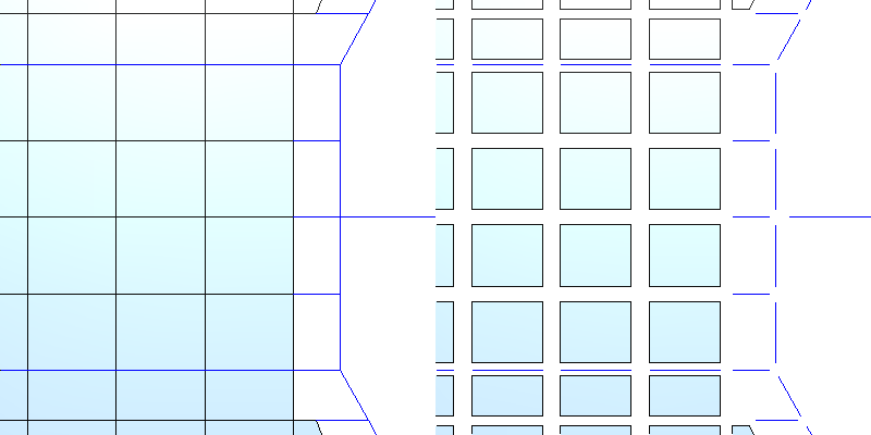
The "shrink" property allows for shrinking of wire elements and element faces. This permits for instance to inspect neighbouring elements having different but coincident nodes, to find overlapping elements, to detect wrongly-connected elements, etc.
Shrinking is enabled in the graphical user interface by activating the corresponding check box. In the Python environment, it is done with
p.shrink = True
The following image shows the wire elements (blue) and shell elements (light blue) of a detailed view of the bridge Finite-Element model. To the left, no shrink is applied. To the right, the elements are shrunken.
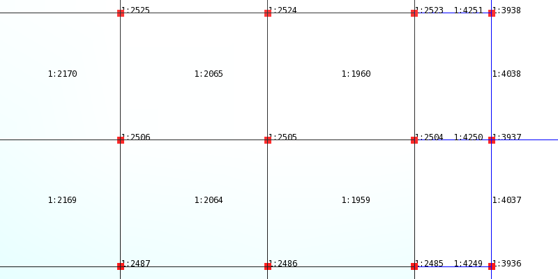
Elements and nodes numbers can be displayed optionally. While the node numbers are displayed near the node locations, element numbers are displayed at the centres of the element faces (since baspl++ displays volume elements by displaying the element faces). The numbers consist of the branch number followed by a colon (":") and the node and element numbers respectively.
It is worth noting that the display of node and element numbers may not only considerably slow down the display performance, but also clutter the displayed image, especially when zoomed out. Thus, these options are best enabled when the model view is zoomed to a detail.
![[Note]](common/images/admon/note.png) |
Note |
|---|---|
|
Node and element numbers are displayed using textures in OpenGL, and at either the node's location or the element's centre or face centre. When element faces are either curved or the viewing perspective is not perpendicular to them, it may well be that the texture will be occluded by the polygons representing the element faces. It thus might be necessary to rotate the model such that the labels become visible again. |
In the graphical user interface, these methods are available on the "Label" sub-page and can be enabled by activating the corresponding check boxes.
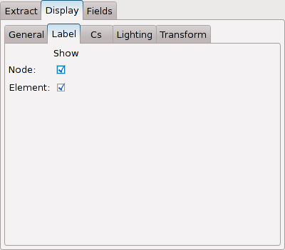
In the Python environment, they are accessed via the "label" sub-object in the following way:
p.label.node.show    = True # activates display of node numbers
p.label.element.show = True # activates display of element numbers
The following figure contains a detail of the bridge Finite-Element mesh (containing nodes, wire and shell elements), with the node and element numbers being displayed.
|
Note |
|---|---|
|
The display methods described in this section are used with Finite-Element meshes for stress analysis. |
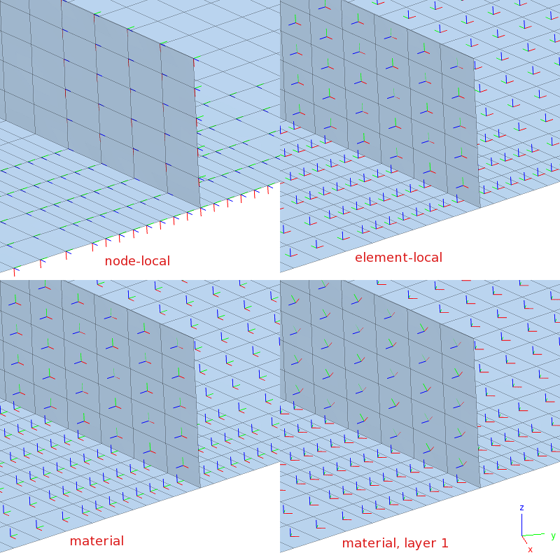
Finite-Element meshes for stress analysis often involve local coordinate systems to allow for more intuitive definition of boundary conditions and material directions. Such coordinate systems may defined at the nodes, for elements, and for materials. In case of laminated materials, there is a coordinate system for each layer of the laminate.
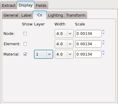
These coordinate systems can be displayed. The local x-, y-, and z-axes are displayed in red, green, and blue, respectively. The line width and length scale factors can be adjusted.
In the graphical user interface, the settings are found on the "Cs" sub-page. The display is enabled by activating the respective check boxes. For the material coordinate systems, the "layer" drop-down combo box permits to select the laminate layer. By default "None" is selected, meaning that the element-material coordinate system is chosen.
|
Note |
|---|---|
|
In laminated materials, the layer coordinate system is usually turned by an angle of e.g. 45 degrees w.r.t. the element-material coordinate system. The choice of layers available corresponds to the set of all layer numbers for the whole mesh. Choosing a high layer number (e.g. 24) will not apply to elements having fewer layers. This does not produce any error, instead, the material coordinate system is not displayed in such cases. |
In the Python environment, display of the coordinate systems is enabled as follows:
p.cs.node.show     = True
p.cs.element.show  = True
p.cs.material.show = True
The "width" and "scale" properties are available:
p.cs.node.width = 2
p.cs.node.scale *= 4
The "material" sub-object has the "layer" property:
p.cs.material.layer = 7
The following figure displays four screen shots of a curved and stiffened composite panel, showing different coordinate systems. Note that the panel is not aligned to any of of axes of the global coordinate system.
When OpenGL-lighting is used (by default), the default settings
for the lighting of the NPart object suffice most
of the time. In some cases however, there might be need to tweak these
settings or to disable lighting altogether. This is described in this
section.
In the graphical user interface, these settings are located on the "Lighting" sub-page.
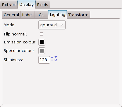
The most important setting is the "mode" property. It defines the lighting mode. By default, this is "gouraud" shading, meaning that the surface normals are averaged, creating the illusion of a smooth surface. The "flat" mode on the other hand uses non-averaged surface normals and is useful for examination of the mesh quality.
In the graphical user interface, the lighting mode is selected via the drop-down combo box labeled "Mode". In the Python environment, the mode is set as follows:
p.lighting.mode = 'gouraud'
p.lighting.mode = 'flat'
p.lighting.mode = None
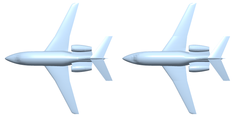
The following figure displays the wall surface of an aircraft. On the left, Gouraud shading is being used, while on the right, flat shading is being used.
|
Note |
|---|---|
|
The normal-averaging procedure used in Gouraud shading requires that
|
When lighting is disabled (p.lighting.mode ==
None), the remainder of the settings described in this
section has no effect.
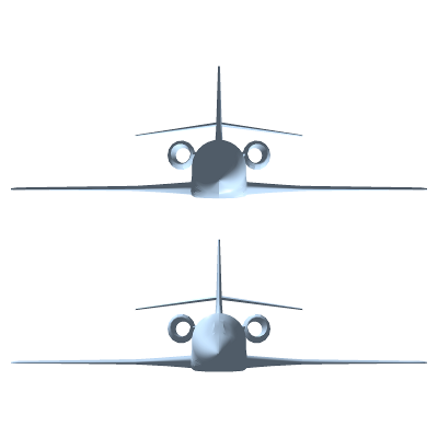
The normal vectors may be flipped (that is, inverting their
signs). The effect can be seen in the following figure, where the
upper NPart object has the normals flipped.
Flipping is enabled by activating the corresponding check box in the
graphical user interface, or in the Python environment
p.lighting.flip_normal = True
Emission and specular colour are by default set to colour-neutral values. They may be changed to any colour. In the graphical user interface, this is done by clicking on the coloured buttons. In the Python environment, the "colour" sub-object contains these properties:
p.lighting.colour.emission = 'blue'
p.lighting.colour.specular = 'green'
The "shininess" property controls the amount of specular reflection. It accepts values between 0 and 128 (default). In the graphical user interface, the values are specified in the corresponding entry widget at the bottom of the "Lighting" sub-page. In the Python environment, this is done as follows:
p.lighting.shininess = 50
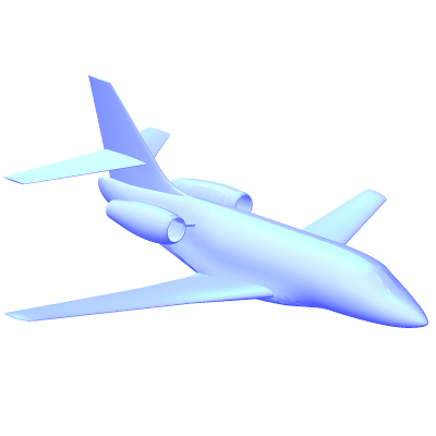
The following figure displays the aircraft model with the settings as in the examples above.
Like any 3D renderer object, an NPart object
can be translated, scaled, and rotated in the Scene
object. This so-called "modelview" applies in the same manner to all
3D objects that have been added to the Scene
object. Sometimes it might be desirable to scale or move one
NPart object differently than the other
NPart objects. This is especially useful where the
same mesh should be displayed twice, with some distance between them.
For half- and quarter-models, the possibility to mirror may also be
useful.
In the graphical user interface, these settings are found on the "Transform" sub-page. In the Python environment, they are accessed via the "transform" sub-object.
Scaling is done via the "scale" property, which is a tuple of three floating-point numbers for the x-, y-, and z-direction, by default (1, 1, 1). In the graphical user interface, the widget consists of three entries, one for each direction. The "*" button at the right of the widget defines if the values are synchronized. In the Python environment the scale property is set as follows:
p.transform.scale = [1, 1, 2]
Translation is defined in Scene coordinates. Thus, the x-axis going to the right, the y-axis going to the back(ground), and the z-axis going up. The units however are those of the mesh. The "translate" property is used in the same fashion as the "scale" property.
p.transform.translate = [0, 0, 15]
Finally, the "mirror" property consists of a list of the following options:
-
nv: Normal view (default). -
xy: Mirror at the xy-plane. -
yz: Mirror at the yz-plane. -
xz: Mirror at the xz-plane. This option is often used with CFD half-models.
In the graphical user interface, the choice is defined via the drop-down combo box. In the Python environment, the "mirror" property accepts a comma-separated character string. It is also possible to supply a list of strings:
p.transform.mirror = 'nv,xz'
p.transform.mirror = ['nv', 'xz']
The following figure illustrates mirroring and translation. The
upper NPart object is translated by 15 units in
z-direction. The lower NPart object is mirrored in
the xz-plane.
