|
|
|
B2000++ is a Finite Element environment for solving solid mechanics, heat transfer and coupled solid-fluid problems. With B2000++, you can predict with a high degree of accuracy the deformation field, the stress field, the buckling behavior, and the temperature distribution of many thin- and thick-walled, metallic and laminated composite structures. The modular architecture allows you to extend its capabilities and to create plug-ins. B2000++ works on Linux, and the source code of B2000++ is released under the GPL version 3 (GPLv3).
B2000++ Pro extends the capabilities of B2000++ to geometric nonlinear analysis, e.g. to predict the static and transient post-buckling behavior, and material nonlinear analysis, including hyperelastic and viscoelastic material models. It can be executed in parallel on shared and distributed architectures with the MUMPS sparse linear solver. B2000++ Pro contains advanced modeling capabilities like the field_transfer coupling method and includes the post-processor baspl++. B2000++ Pro includes installation support and one year of updates. Customers who purchase B2000++ Pro have access to the source code repository and to the suite of verification tests.
For assembly and stress recovery, the symmetric multi-processing (SMP) capabilities of modern CPUs are exploited. The integration with external state-of-the-art sparse matrix solvers, in addition to B2000++'s own direct multifrontal matrix solver, enables parallel matrix resolution for SMP and - for workstation and site licenses in combination with B2000++ Pro - for distributed computing via MPI. This results in a high level of parallelism for an implicit FE solver, ideally suited for the analysis of large and detailed FE models.
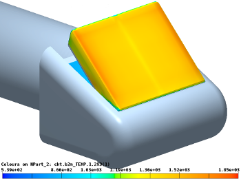
Thermal analysis simulation capabilities include conduction, convection and radiation, steady-state and transient conditions with two- and three-dimensional elements. Materials can depend on temperature and/or time. For radiation between different parts of the FE model, B2000++ Pro can automatically calculate the visibility factors from the geometry. Thermal analysis can be coupled to solid mechanics analysis or CFD solvers with the FSCON/FSI multi-physics coupling tools. [more]
All beam, shell, and solid elements support laminated composite materials and per-layer thermal expansion coefficients. For the beam elements, arbitrary cross sections can be made from 2D meshes, with B2000++ Pro automatically calculating the section properties. The shell elements use the MITC (Mixed Interpolation of Tensorial Components) formulation and, for linear elastic materials, perform the through-the-thickness integration a priori analytically, resulting in fast assembly. Stresses are recovered for each layer at the Gauss points in the shell and solid elements. For the latter, a large range of different quadrature rules can be chosen from.
For the accurate prediction of damage onset, a comprehensive set of failure criteria for metallic and composite structures is available: Maximum stress, maximum strain, von-Mises, Tsai-Hill, Tsai-Wu, Hashin (in-plane and 3D), and LaRC04 (in-plane). And in conjunction with failure criteria, stresses can be filtered to effectively reduce the amount of data that will be stored on the analysis database.
In combination with solid elements, delamination growth and debonding can be simulated with B2000++ Pro by means of VCCT elements and the cohesive zone material model. Solid elements and shell elements can be kinematically coupled for nonlinear global-local analysis with SMR's high-fidelity common-refined mesh algorithm.
Except for the definition of the nonlinear analysis parameters, there is no additional FE modeling effort required when going from linear to nonlinear analysis, since the formulations of the truss, beam, shell, solid, rigid-body, and even point-mass elements are nonlinear, and therefore any FE model that was made for linear analysis can be used for nonlinear analysis as well.
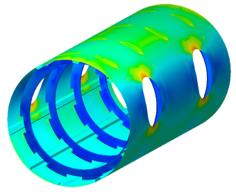
The linearized pre-buckling solver allows for a quick estimation of the initial buckling load. Depending on the type of structure, the predicted buckling load may be verified by means of an incremental analysis.
B2000++ Pro's quasi-static incremental solver offers the following increment control strategies: Load control with artificial dissipation, state control, hyperplane control (Riks method), local hyper-elliptic control (Crisfield method). A number of different analysis solution parameters allow for fine-grained control over the Newton strategy and the detection of convergence and divergence. Boundary conditions can be applied individually in different analysis stages, and they can be scaled by means of mathematical expressions.
The implicit transient solver available in B2000++ Pro makes use of the multi-step backward-differential time integration shema which gives unconditional nonlinear stability for the schema of order 2. Variable time-stepping is enabled with the Nordsieck transformation method, and the step size is controlled with a local error estimator that is obtained with Milne's method. The solver also implements a strategy to re-use the factored matrix between different steps if the convergence of the Modified Newton iteration is good. This generalization of the Modified Newton idea is essential because the step size is not only controlled by the accuracy of the matrix - like for the static non-linear solver - but also by the local error of the time integration scheme. The solver is therefore suited for the simulation of highly nonlinear dynamic phenomena, such as buckling. Like for the quasi-static solver, boundary conditions can be individually staged, and they can be scaled by means of mathematical expressions.