6. Verification and Examples
In the present version the Simples tests verify the functioning of
Simples with B2000++ (tests under directory tests/b2000pp) and
the internal functioning of Simples (tests under directory
tests/internal). The tests can be launched from their
respective directories with the b2testrunner application:
b2testrunner [-j NPROC] .
In case of failure, clean up with
find . -name "tmp_b2test*" -exec rm -r {} \;
6.1. B2000++ Tests
Note that many Simples scripts are executed in the B2000++ system
tests under the $B2EXAMPLES and $B2VERIFICATION folders, thus
also serving as Simples tests.
Specific B2000++ Simples tests are found under tests/b2000pp,
some of the documented here or in the respective test scripts.
6.1.1. NBC Generation
Location of test: tests/b2000pp/boundary_conditions/truss
Tests the modification of applied forces with
Simples. The example is taken from the BDF converter
verification case bdf_truss. The
Simples test script run.py does:
Create a
NBCforcesorNBCvaluesset and solve the problem.Replace the original set with modified values.
Solve the problem again.
This script is an adaptation of a DLR bug report.
6.1.2. Section Stress Test
Localtion of test: tests/b2000pp/beam_sections/stresses/bar
Tests the BeamStressField class with a I-profile
cross-section. The test run.py does:
Launch a linear static analysis of a cantilever beam model
beam.mdlcomposed ofBx.S.RSbeams.For specific loading conditions, the test extracts the
BeamStressFieldand computes the stresses of the bar section at the pre-defined section stress points (see figure). It then compares the stresses with analytical ones.
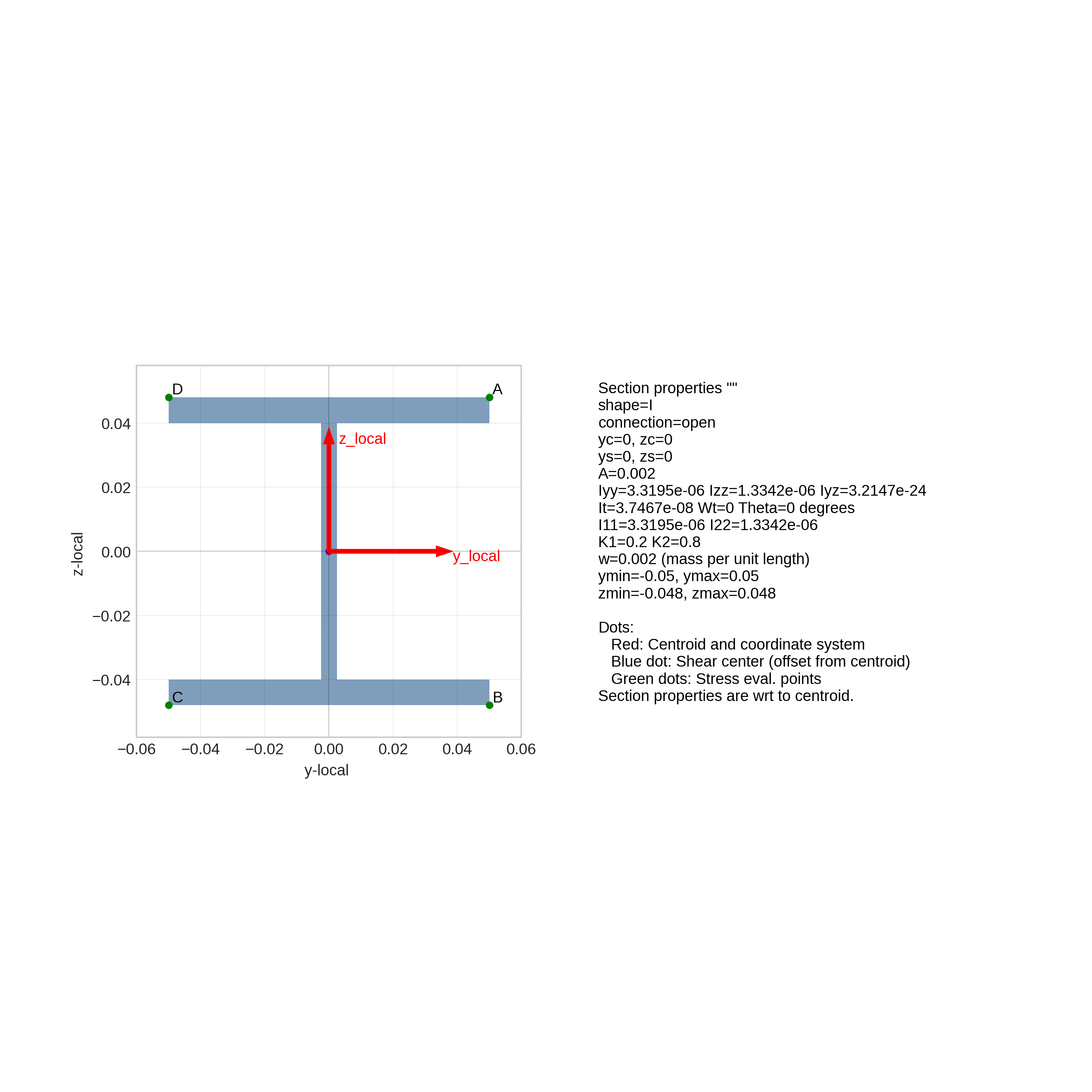
I-profile test section stress evaluation points A, B, C, and D.
Note
In the current version no failure index is computed due to a bug.
6.1.3. Section Properties Calculation Tests
Location of test: tests/b2000pp/beam_sections
Tests section properties of pre-defined and user-defined sections with
the Simples bcs module. The test also generates section plots (png
files). Run the test with the b2testrunner or one by one with
(example):
python3 l_section_test.py
Check result (must be 0), bash example:
echo $?
Remove the generated files
make clean
6.2. Other Tests documented locally
tests/b2000pp/beam_sections/stresses/sectionproperties
tests/b2000pp/applications
tests/b2000pp/b2util
tests/b2000pp/boundary_conditions
tests/b2000pp/case
tests/b2000pp/fields
tests/b2000pp/material
tests/b2000pp/model
6.3. Internal Tests
6.3.1. Spline Interpolation tests
Note
Location of test: tests/internal/splines
Simples spline interpolation class tests. The tests do not check if the generated interpolation curves are correct but they generate relevant plots.
spline2.py approximates a series of data points with
interpolation.BSplinePCurve, both in \(R^2\) (y, z plane) and in \(R^3\)), and creates the graphspline2.svg.

Spline interpolation test 2: Data Points and interpolated curve.
spline3.py approximates an analytical function defined by points with
interpolation.BSplinePCurvein \(R^2\) and creates the graphspline3.svg. The example comes from scipy.

Spline interpolation test 2: Data Points (red) and interpolated curve (blue).
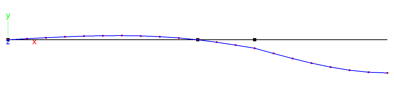
bezier.py approximates a circular arch defined in x-y plane with
interpolation.BezierCurvein the interval [pi/2,0] with 5 optimally placed control points points.Origin of data: Seebezier.py.

Bezier curve interpolation test 3: Data Points (red) and interpolated circular arc (blue).
6.3.2. Compare Curve Test
Location of test: tests/internal/util
The `` test checks the function
simples.util.compare_curve1(). It generates 2 similar curves and
compares them with the util.compare_curve1 function. Execute test
with
python3 compare_curve.py
The test generates the graphs compare_curve.png and compare_curve.svg:

Compare curve example.
6.3.3. Compare Floats Test
Note
Location of test: tests/internal/util
internal/util
The compare_floats.py test checks the function
simples.util.compare_float(). Execute test with
python3 compare_float.py
6.4. Minimodeler Examples
6.4.1. Cook Membrane Problem (Modeler)
Location of verification case: $B2EXAMPLES/minimodeler/cook_membrane
This case is equivalent to the Cook Membrane Cook Membrane Problem verification case, with the difference that the FE mesh is generated with the Simples modeler.
The Cook membrane problem is a classical test case for linear static analysis named after the author, R. D. Cook [cook1974] who first reported it. The structure consist of a trapezoidal surface in the x-y plane (see figure below and MDL input file for dimensions and material constants).

Cook membrane: Mesh generated by Modeler (red: Modeler Points). FE mesh (right).
The structure is clamped along the edges E4 and it is loaded by a edge traction load along the right vertical edge with a total load of 1 in the y direction.
The problem is solved with a single Simples script file:cook_membrane.py, which
generates the Brep model,
creates the FE mesh,
generates the B2000++ MDL input file.
Solves the problem with B2000++,
Checks the result.
An extract of the file:cook_membrane.py illustrates the generation of the Brep model and the FE mesh:
NE = 64 # Number of elements in u and v

m = si.Model('cook_membrane',  'nd')
mm = m.get_modeler()

# Line load along edge (edges et) "e4": Total force=1 over length=16.
pressure = 0.1/16.0

mm.point('p1', (0, 0, 0))
mm.point('p2', (48, 44, 0))
mm.point('p3', (48, 60, 0))
mm.point('p4', (0, 44, 0))

e1 = mm.edge("e1", "sline", ( 'p1', 'p2'), ncells=NE)
e2 = mm.edge("e2", "sline", ( 'p4', 'p3'), ncells=NE)
e3 = mm.edge("clamped", "slin e", ('p1', 'p4'), ncells=NE)
e4 = mm.edge("e4", "sline", ( 'p2', 'p3'), ncells=NE)

surface = mm.surface4("surface", "coons", 'p1', 'p2', 'p3', 'p4')

t0 = time.time()

# Make the FE mesh (mesh only  with generic elements)
mm.make_fe_mesh()
The solution visualized with baspl++ is displayed below
(see script bv-deformed-fe-mesh.py:
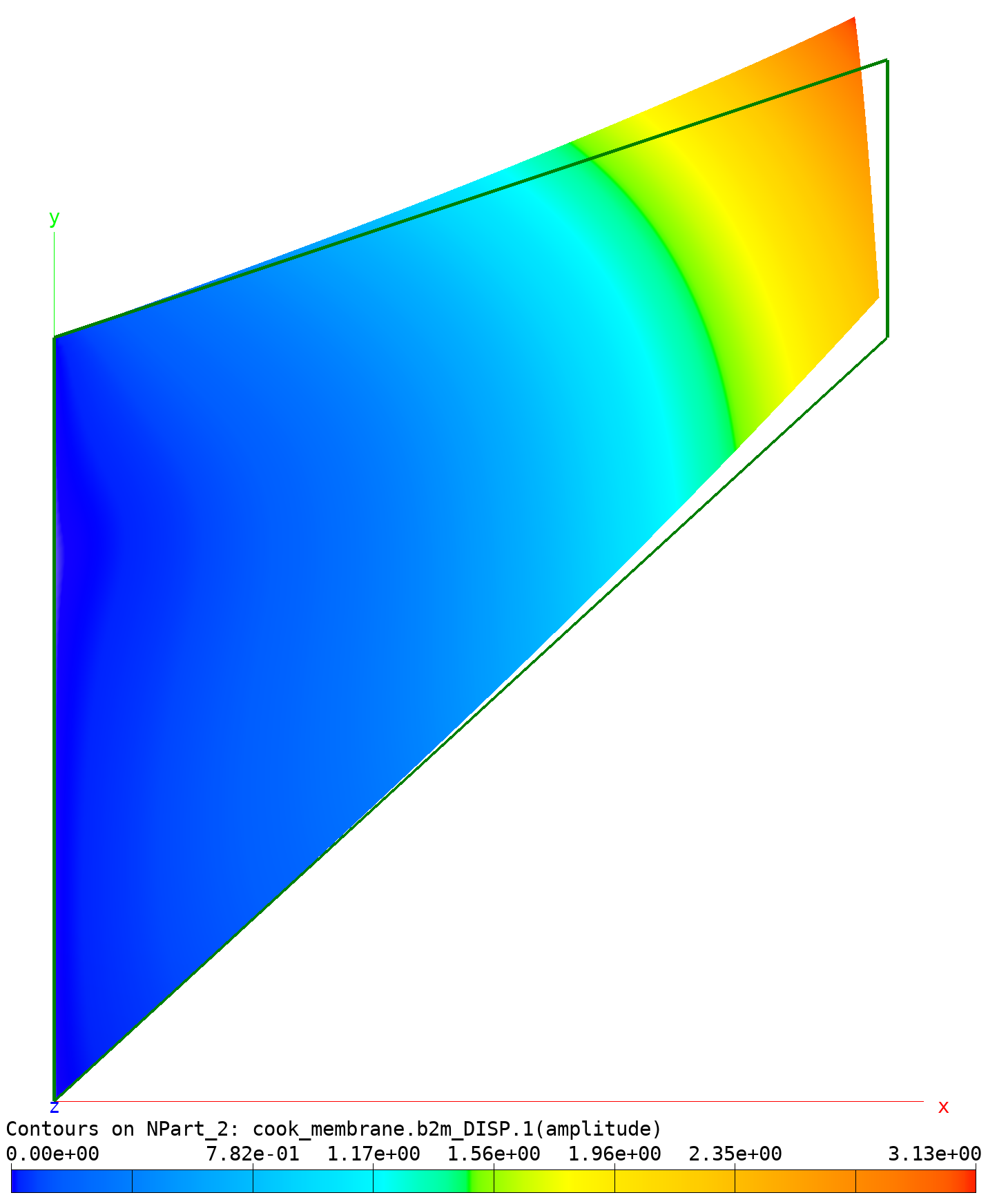
Cook membrane: Deformed mesh (amplitude colored) and undeformed mesh.
6.4.2. Axially Compressed Cylinder
Location of example case: $B2EXAMPLES/minimodeler/cylinder
This test case demonstrates the automatic parametric mesh generation and convergence testing of buckling analysis of a cylinder.
The model is a thin cylinder made of aluminum with the following properties:
Radius R [mm] |
250 |
|---|---|
Length L [mm] |
500 |
Thickness T [mm] |
0.5 |
Young’s modulus E [N/mm2] |
70000 |
Poisson ration NU |
0.33 |
The mesh is generated such that the cells are approximately quadratic. The number of cells in axial direction (NAXIAL) and radial direction (NRADIAL=4*NAXIAL) vary for the convergence study.
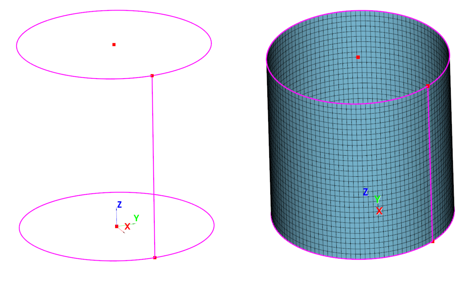
Buckling of cylinder: MiniModeler brep (left) and FE mesh (right).
The first part of the test concerns linear buckling. The cylinder is generated with the Minimodeler by defining the lower and upper circle of the cylinder. Meshing is automatic: The figure below shows the Minimodeler Brep definition of the cylinder and the meshed cylinder.
The Python script buckling.py solves for 1 specific mesh
configuration. See comment.
The buckling shape can be plotted with the bv-buckling-modes.py
script:
baspl++ bv-buckling-modes.py
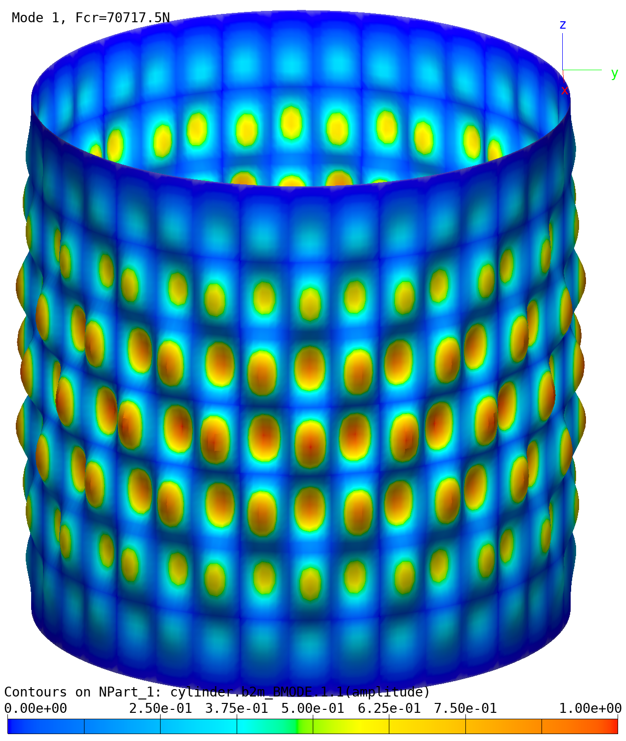
Buckling of cylinder: Buckling mode 1.
Postbuckling: Documentation in preparation.
6.4.3. Beam with pin-joint
Location of verification case $B2EXAMPLES/minimodeler/gerbertraeger
The model consist of a beam that spans over 2 segments (see figure below). The first segment of the beam is supported at both ends. The right end of the second segment reflects symmetry. A pin-joint is placed such that the beam becomes ‘statically determinate’, preferably at a place where the moment is 0 for the dominating load case. The principle is called after the German engineer H. G. Gerber who designed bridges in the 19th century.

Beam with pin-joint: Mesh and supports.
The dimensions, material parameters, and the load can be found in the respective MDL input files.
Two models are defined:
End-releases at one element attached to the pin-joint (
releases.mdl).Duplicated nodes at the pin-joint location. The nodes are coupled with linear constrains, except for the rotation \(R_{z}\), thus modeling the pin-joint (
linc.mdl).
Beam with pin-joint: Deformed beam shape (amplified).
The deformations with or without pin-joint are quite close. This is to be expected, because the pin-joint is near the place where \(M_{zz}=0\) in the system without pin-joint. Note that this is the general idea with the Gerbertraeger: Place the pin joint where the moment for the main load case, usually the weight, is 0 in a system without pin-joint. The table below shows the displacement \(D_{z}=0\) under the load P:
Item |
Release |
Linc |
|---|---|---|
DZ Symmetry |
-0.1102 |
-0.1102 |
Reaction Force A |
-150 |
-150 |
Reaction force Fz at B |
650 |
650 |
Moment My at B |
-3500 |
-3500 |
The moment \(M_{zz}\) and the stress \(\sigma_{xx}\) along the beam (end release model) are plotted in the figure below. At the location of the pin joint (x=13) the moment must be 0 for both elements attached to the node at x=13.

Moment \(M_{zz}\) along beam x-axis. Results identical for both models.

Moment \(M_{zz}\) along beam x-axis. Results identical for both models.

Failure index (von Mises) along beam x-axis. models.
The moments, stresses, and failure index graphs were obtained with the
script plot_moments_stresses.py. Stresses can be printed with
the script stresses.py.
6.4.4. Plate under normal pressure
Location of example case $B2EXAMPLES/minimodeler/plate_pressure
A rectangular simply supported plate in the x-y-plane defined by the
four points p1 to p4 is subject to a uniform normal
pressure.
  "p3"         "e2"         "p2"
     +----------------------+
     |                      |
"e3" |       "plate"        | "e1"
     |                      |
     +----------------------+
  "p0"         "e0"         "p1"
The file test.py creates the mesh runs the analysis and
examines the results. Execute the test with
python3 plate.py [order]
Element order (optional) is 1 (Q4 elements) or 2 (Q9 elements).
View the deformed plate and stresses \(\sigma_{xx}\) with baspl++:
baspl++ bv-disp-stress.py
6.4.5. Tensile Strip with Hole
Location of example case $B2EXAMPLES/minimodeler/tstrip_with_circular_hole
Stresses and the stress intensity factor in a aluminum tensile strip with a circular hole are computed. The stress intensity factor is computed in a post-processing step. The analytical solution \(\sigma_{max}\) for the stress intensity factor is
where \(P\) is the force with the strip is pulled, \(D\) is the width of the strip, \(t\) the thickness of the strip, and math:r the radius of the hole.
The FE model consist of a single branch generated with 3 Simples surface patches and meshed with either Q4 or Q9 shell or 2D elements:
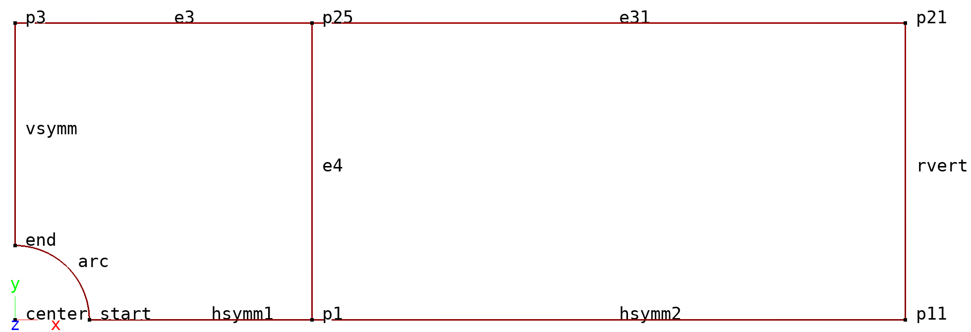
Tensile strip: Modeler Brep mesh.
The width of the strip \(D=25.4\), the thickness \(t=.616\), and the radius of the circular hole \(r=3.18\). The strip is clamped at one end and loaded with a ‘displacement load’, i.e an essential boundary condition, at the other end, where a the DOF 1 (x-direction) is constrained to 0.013. To obtain the total reaction force and to compute the theoretical solution a Python script is included.
To run the script type:
python3 tstrip.py [order]
where the option order set to 2 will generate a linear Q mesh
(default) and set to 3 a quadratic Q (Lagrange) mesh.
The linear analysis is performed with Q shell or 2D elements. material with \(E=69 \cdot 10^3\) and \(\nu=0.3\) and the failure stress is assumed to be \(\sigma_{f}=138\). Note that the material has no influence on the stress concentration factor, as long as the material is isotropic and elastic and the calculations are linear.
The Python post-processing program extracts the reaction forces at the constrained nodes, sums them up to get the total reaction force \(P\), and calculates the theoretical \(\sigma_{max}\) for the given force:
Total reaction force P = 742.857 N
Effective Area = 24.904 mm^2
Theoretical stress concentration factor h = 2.422
Sigma_nominal P/A = 29.828 MPa
Sigma_max_theoretical = h*Sigmal_nominal = 72.236 MPa
Sigma_max_computed = 70.755 MPa
Error (percent): 2.050
Area = 475.928 (analytical area = 475.928)
The stress plot as illustrated below is obtained with the
baspl++ bv-vmises-contour.py
shell command.
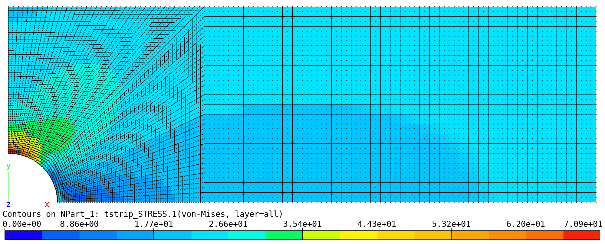
Tensile strip: von Mises stress (max of element), Q9 mesh.