4. Using Simples Classes

Note

Still in preparation.

Simples consist of a collection of Python modules and classes for accessing and manipulating B2000++ FE models. In addition, it provides a FE mesh modeling module (prototype) for generating FE meshes and B2000++ input files from this module. Simples is designed such that most of the functionality is independent of the underlying data manager.

This chapter explains the functioning of the modules and classes with examples. All Simples examples consist of Python scripts.

4.1. The Model

The Model is the top-level class for processing B2000++ models. It contains references to the meshes, solutions, boundary conditions. A B2000++ model is created or opened with the Model class:

import simples as si
model = si.Model('scordelis_lo_roof.b2m)

To work with meshes, get a reference to a branch (mesh) object identified by a positive integer (usually branch or mesh 1):

branch = model.get_branch(1)

and operate on the Branch object. Example: Show element parameters of element 23

branch.get_elem[8].show()

results in

Element 8:
Internal identifier iid=7
Centroid=[ 1.08944678 24.95243373  1.5625    ]
Connectivity (internal ids) conn=[ 7  8 17 16]
Element type name elname=Q4.S.MITC.E4
Element family member=Q4
Internal type ityp=97
Material identifier=1
Property identifier pid=0

4.2. Solution Cases

The Case objects describe the solution field parameters of solution case(s), such as

• Analysis type

• DOF solution field names: dof (solution field), dofdot (time derivative of DOF), dofdotdot (time derivative of time derivative of DOF)

• Initial DOF solutions flags dofinit, dofdinit (transient analysis)

• Right-hand side vector field name (nbc’s)

• Residuum solution field name

• Gradients solution field name(s), i.e. sampling point fields

Case objects are loaded by the and can be retrieved with the Model functions get_case(), get_cases(), and get_cases_lists()>(). The get_case() returns a reference to a defined case object of a model. Example: Get the nonlinear solution steps identifiers (cycles) of the case 1:

cycles = model.get_case(1).cycles

4.3. Boundary Conditions

The boundary condition definitions described herein closely follow the B2000++ MDL nbc specification.

Boundary conditions are additive, i.e values of the components can be accumulated. The add() methods will add values to any existing values, while set() overwrite any existing values with the new ones.

4.4. Solution Fields

Simples fields refer to discrete (solution) fields defined at mesh nodes or in elements. Fields are usually Solution Fields produced by the B2000++ solvers or by any other program producing solution fields.

Simples solution fields allow for using aliases which are more descriptive that the standard B2000++ generic field names:

Field name aliases (not case sensitive)

displacements	Displacements at nodes (3 components).
forces	Forces at nodes (3 components).
heat	Heat at nodes (1 component).
moments	Moments at nodes (3 components).
reaction_forces	Reaction forces at nodes (3 components).
reaction_moments	Reaction Moments at nodes (3 components).
rotations	Rotations at nodes (3 components).
temperatures	Temperatures at nodes (1 component).

The case objects contains references to the solution fields.

4.4.1. Node or DOF Fields

The simples.fields.NodeField object contains a field defined at the mesh nodes, usually a DOF field, such as a displacement field or a temperature field, for a given case and cycle. Values can subsequently be extracted or inserted with the following methods:

• To access all values, make use of the values pointer of the object. It points to the ‘raw’ numpy array of nrows*ncolumns.

• To extract a range of values at selected nodes, make use of the get function.

• To extract the values of a single node, address the field with the [key] operator, where key is the external node identifier.

Note that the NodeField loads the complete field from the database. If a single row is to be extracted please make use of the simples.Model() method get_node_field1().

4.4.2. Element Fields

The simples.fields.ElementField contains element-wise defined fields for a given case and cycle. Similar to node fields, the number of values or data columns of each element is constant (element with values varying from element to element are stored in Sampling Point fields).

4.4.3. Sampling Point Fields

The simples.fields.SamplingPointField class contains element-wise defined derived fields, such as such as strains, stresses, section forces, heat flows, etc. for a given case and cycle. Values are defined at specific evaluation (sampling) points within an element. Since element solution data is heterogeneous the number of evaluation points data vary from element to element. But the number of values at all evaluation points is constant and equal to the number of field components.

The B2000++ sampling point field database storage scheme allows for accessing the sampling point field values, the sampling point field coordinates and more.

The numpy array for one element as returned by the get functions is 2-dimensional array

values[n, ncomp]

where n is the total number of sampling points and ncomp the number of field components at each sampling point. The number of sampling points depends on the element integration scheme and on the material type.

The simplest way of identifying the sampling points is to call the method get_icoor(). It returns an array icoor containing the positions of the n sampling points, expressed in natural coordinates \(\theta^{1}\), \(\theta^{2}\), and \(\theta^{3}\) ranging from -1.0 to 1.0.

If the material type is not layered, i.e. the material type is not LAMINATE, the field array values contains 3 sub-layers one after the other, at the natural coordinate system z coordinates \(\theta^{3}=-1.0`\), \(\theta^{3}=0.0`\), \(\theta^{3}=1.0`\). Each sub-layer contains m values, where m=4 for the 2x2 scheme, where m=9 for the 3x3 scheme.

Non layered material: Stress evaluation point definitions through element thickness.

If the material type is layered, i.e. the material type is LAMINATE, the field array values contains all sub-layers one after the other, starting at z=-1.0 and up. The first and the last layers contain 3xm values at the natural coordinate system z coordinates \(\theta_{rel}^{3}=-1.0\), \(\theta_{rel}^{3}=0.0\), and \(\theta_{rel}^{3}=1.0\), whereas the intermediate layers contain m values at \(\theta_{rel}^{3}=0.0\). math:theta_{rel} means that the natural coordinate system is relative to the layer (thickness).

Layered material: Stress evaluation point definitions through element thickness.

class SamplingPointField(model, name, branch=1, case=1, cycle=None, subcycle=None, subcase=None, metadata=None)

Bases: FieldBase

Creates and loads a field defined at the element sampling points (also referred to as ‘integration points’. Sampling point fields contain values produced by the B2000++ solver, such as strains, stresses, section forces, etc.

Parameters:

• model (Model) – Model object containing the sampling point field.

• name (str) – Field name. Field names depend on the B2000++ solver.

• branch (int) – Identifier of branch to be selected. The default value is 1.

• case (int) – Solution case. The default case is 1.

• subcase (int) – Solution subcase. The default is None.

• cycle (int) – Load or time increment cycle. The default cycle is 0.

• subcase – Solution subcase or buckling or free vibration analysis mode. The default is None.

Returns:

Array containing sampling point field values for all sampling points of element(s).

get_i(iid)

Extracts all values for the element specified by its internal identifier iid.

Parameters:

iid (int) – Internal element identifier.

Returns:

Array of rows containing the values for all integration points of the specified element or None (see numpy return value). All values are floats.

get(eid)

Extract all values for the element specified by its external identifier.

Parameters:

eid (int) – External element identifier.

Returns:

Array of rows of floats containing the values for all integration points of the specified element or None (see numpy return value). All values are floats.

get_icoor_i(iid)

“Get the element natural coordinates of the integration points for the element specified by its internal identifier. See also ref:SamplingPointField <field.spf.arrays>.

Parameters:

iid (int) – Internal element identifier.

Returns:

Array of floats containing the element (natural) coordinates or None (see numpy return value). All values are floats.

get_icoor(eid)

Get the element natural coordinates of the integration points for the element specified by its external identifier. See also ref:SamplingPointField <field.spf.arrays>.

Parameters:

eid (int) – External element identifier.

Returns:

Array of floats containing the element (natural) coordinates or None (see numpy return value). All values are floats.

get_layers_i(iid)

Get the material layers of the integration points for the element specified by its internal identifier. See also ref:SamplingPointField <field.spf.arrays>.

Parameters:

iid (int) – Internal element identifier.

Returns:

Array containing material layer definitions or None (see numpy return value). All values are floats.

get_layers(eid)

Get the material layers of the integration points for the element specified by its external identifier. See also ref:SamplingPointField <field.spf.arrays>.

Parameters:

eid (int) – External element identifier.

Returns:

Array containing material layer definitions or None (see numpy return value). All values are floats.

get_min(colname)

Compoutes the overall minimum value of a column (component).

Parameters:

colname (str) – Name of column or, if colname is an int, column (component) index. Note that column indices start with 0.

Returns:

List containing [eid, [x,y,z], ip, value], where eid is the sample field external element number,`` [x,y,z]`` are the sampling point global cooordinates, ip is the integration point number, and value is the minimum of all values of the column colname.

Raise:

Exception if column colname not found.

get_max(colname)

Searches the overall maximum value of column (component).

Parameters:

colname (str) – Name of column or, if colname is an int, column (component) index. Note that column indices start with 0.

Returns:

List containing [eid, [x,y,z], ip, value], where eid is the sample field external element number,`` [x,y,z]`` are the sampling point global cooordinates, ip is the integration point number, and value is the maximum of all values of the column colname.

Raise:

Exception if column colname not found. of range.

get_layer_count(eid)

Get the layer items count list for each layer. The list items are tuples

(i, n, nsub)

where i is the layer number (starting at 0), `` n`` the total number of items (stress, strain,…) arrays for that layer, and nsub the number of sub-layers. The tuples are sorted in ascending values of i. See also ref:SamplingPointField <field.spf.arrays>.

Parameters:

eid (int) – External element identifier.

Returns:

List of tuples (i,n,nsub), see above, or None.

4.4.4. Beam Stress Fields

A simples.fields.BeamStressField class contains element-wise defined sampling point fields, such as beam forces and moments for a given case and cycle. Derived quantities, such as stresses and strains defined at beam sections along the beam local x-axis for a given case and cycle, are computed on request: As beam Section stress computation is not yet included in the B2000++ solver, the beam section stresses must be computed in a post-processing step from element forces and moments computed by the B2000++ solver. The Beam Stress Fields class computes the section stresses and optionally, the failure index.

The stress evaluation scheme for beam section is implicit for pre-defined beam sections, i.e stresses are computed at the spoints defined by the MDL beam_section beam property definition command. For beam section properties defined by the MDL beamconstants beam property definition command the points are user-defined.

class BeamStressField(model, branch=1, case=1, cycle=0, subcycle=0, subcase=None, metadata=None)

Bases: FieldBase

The BeamStressField object STRESSES_BEAMS loads beam element section forces SECTION_FORCES and section moments SECTION_MOMENTS and computes section stresses for a single given case. The longitudinal stress due to the axial force and due to bending and, if available, the torsional stress st are computed. If available, the failure index is computed.

Parameters:

• model (Model) – Model object containing the node field.

• name (str) – Field name. Field names depend on the B2000++ solver. Some pre-defined names and aliases are available.

• branch (int) – Identifier of branch to be selected. The default value is 1.

• case (int) – Solution case. The default case is 1.

• subcase (int) – Solution subcase. The default is None.

• cycle (int) – Load or time increment cycle. The default cycle is 0.

• subcycle (int) – Load or time increment subcycle. The default subcycle is 0.

get_forces(eid)

Returns section forces for a single element identified by its external identifier.

Parameters:

eid (int) – External element identifier.

Returns:

A numpy array containing section forces (Fx, Fy, Fz) for all integration points or (see numpy return value). All values are floats.

get_forces_i(iid)

Returns section forces for a single element identified by its internal identifier.

Parameters:

iid (int) – Internal element identifier.

Returns:

Numpy array containing section forces (Fx, Fy, Fz) for all integration points or None (see numpy return value). All values are floats.

get_moments(eid)

Returns section moments for a single element identified by its external identifier.

Parameters:

eid (int) – External element identifier.

Returns:

Array containing section moments (Mx, My, Mz) for all integration points or None (see numpy return value). All values are floats.

get_moments_i(iid)

Returns section moments for a single element identified by its internal identifier.

Parameters:

iid (int) – Internal element identifier.

Returns:

A numpy array containing section moments (Mx, My, Mz) for all integration points or None (see numpy return value). All values are floats.

get_stresses(elset=None)

Computes stresses for all integration point sections and for all stress evaluations points of one or more elements identified by their external element identifiers.

Parameters:

elset (list) – External element identifier(s). int or (list, tuple, numpy intarray. If set to None the stresses of all beam elements will be returned. If a list of elements is specified the stresses of all elements will be returned, provided they are beam elements.

Returns:

List of helper classes BeamElementStresses containing the stresses and the optional failure index of the selected elements. One BeamElementStresses object per processed element is returned in the list if no errors occurred. Note: Do no check for None, since the function returns a list!

4.5. Formatting Data

The data formatter classes are helper classes for extracting and for formatting and tabulating of specific datasets. The b2browser data browser makes us of the data formatter classes.

Formatter classes load specific data. Specific methods allow for getting the data in viewable form. Example: Format the buckling mode data, i.e. the eigenvalues and the critical loads, from a buckling analysis. The example Python code below is taken from the Buckling of Composite Plate example.

import simples as si
model = si.Model('demo')
formatter = si.formatdb.FormatBucklingLoad(model, case=1)
print(formatter.format())

produces the output

Eigenvalues and buckling loads, case 1

Total reaction force F=(-158593, 2.50111e-12, -3.66168e-15), amplitude Famp=158593

        Mode       Lambda   Crit. load
           1      0.01718         2725  *
           2      0.03948         6262  *
           3      0.05028         7973  *
           4      0.06912    1.096e+04  *
           5      0.08614    1.366e+04  *
           6       0.1099    1.743e+04  *
           7       0.1128    1.789e+04  *
           8       0.1335    2.117e+04  *
           9       0.1628    2.582e+04  *
          10       0.1632    2.588e+04  *

Lambda (eigenvalue): if > 1 no buckling, < 1 buckling, marked by *
Critical load: F * Lambda (if F != 0)
Reaction force: Sum of reactions due to EBC and NBC

4.6. Beam Cross Sections

The BeamCrossSection class and its derives classes compute beam cross section properties of thin-walled sections defined by segments. There are a number of predefined sections (not necessarily thin-walled), such as box, tube, bar, rod, L-, I-, C-shaped section.

A thin-walled section is defined by one or more segments to be defined. A segments is a list containing

(yzt, att, params)

where yzt[n,3] is an array containing the segment mid-point coordinates y, z, and the thickness t for each of the n points defining the segment. att is a string describing the segments geometry: o means open line, c means closed line (the last point of the array is identical to the first one). params is an optional dictionary containing segments attributes, such as density.

Closed cross sections defined by several segments must specify the outer segment as the first segment. The fist segment of the closed polyline is then used to compute the torsional constant.

Some predefined section classes are available:

• Bar (rectangular), see simples.bcs.BeamCrossSectionBar

• Box, see simples.bcs.BeamCrossSectionBox

• C-shaped profile (“channel”), see simples.bcs.BeamCrossSectionC

• Constants (defined by section constants), see simples.bcs.BeamCrossSectionConstants

• I-shaped profile, see simples.bcs.BeamCrossSectionI

• L-shape section, see simples.bcs.BeamCrossSectionL

• Rod (circular section), see simples.bcs.BeamCrossSectionRod

• Tube: Thin-walled circular tube section, see simples.bcs.BeamCrossSectionTube

4.7. Create Graphs

The Graph2 plot class is a wrapper for the Matplotlib and it allows for plotting of x-y data extracted from the database. The objects are derived from Matplotlib. Thus, all functionality of Matplotlib is available.

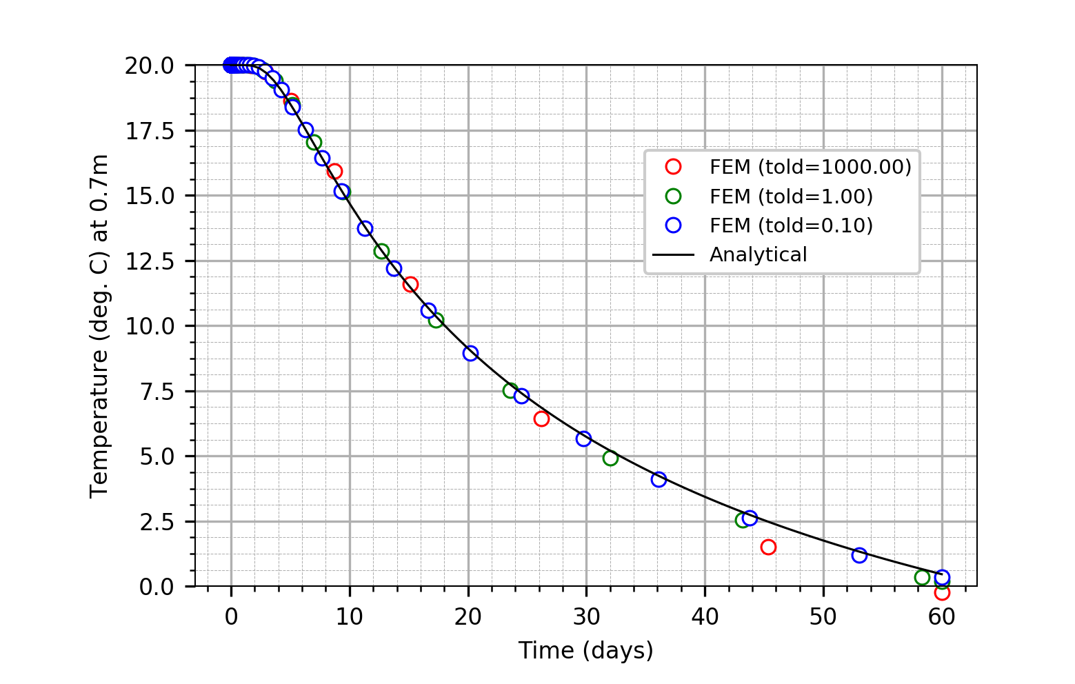
Example: Plot temperatures as a function of time for different solution parameters. The Python example code is taken from the non-stationary heat transfer example example:

g = si.Graph2() # Create a graph
g.axes_label_x='Time (days)'
g.axes_label_y='Temperature (deg. C) at 0.7m'
# solutions is a list ((xvalue, yvalue), ...)
for values, color in zip(solutions, ('red', 'green', 'blue')):
    x = si.util.scale(values[0], 1.1574074074074073e-05)
    line = g.add_line(x, values[1]), markeredgecolor=color, linewidth=0,
                     marker='o', label='FEM (told=%.2f)' % value[2])

# Add analytical value to graph (the function for the theoretical
# value not listed here)
xy  = theor_value(0.7, float(60 * 60 * 60 * 24), 100)
line = g.add_line_xy(xy, label='Analytical', color = 'black')
g.axes_minmax_y = (0.,20.)

# Create figure
g.add_legend(pos=(.6,.6))
g.save('temperature.png')

4.8. The FE Modeler

In preparation.

4.9. Utilities

4.9.1. The Modal Solver

The B2000++ modal transient solver integrates the equations of motion by the modal transformation. The resulting independent equations are then integrated in the time domain with the Newmark method, and transformed back in \(R^3\), see the text book by Clough and Penzien [clough].

A modal transient analysis example of is presented in the examples collection.

4.9.2. Interpolation of Curves

The interpolation module contains interpolation utility classes, built on the scipy interpolation functions:

• Spline curve interpolation simples.interpolation.Spline1

• Parametric B-spline curve interpolation simples.interpolation.BSplinePCurve

• Bezier spline curve interpolation simples.interpolation.BezierCurve

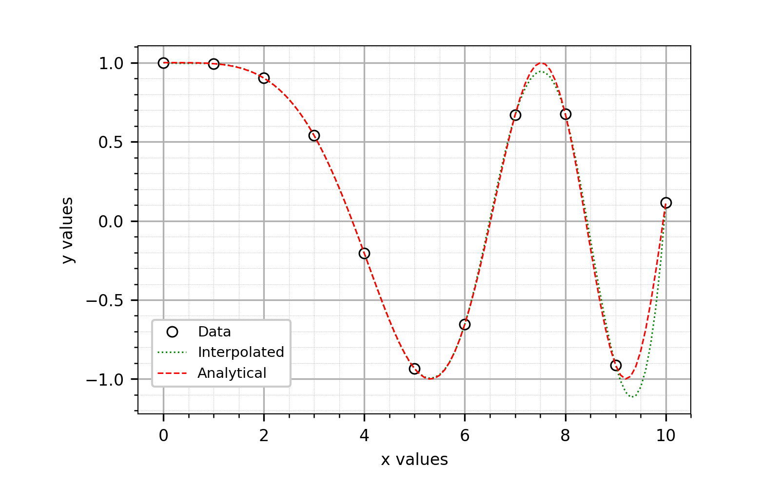
ExampleSpline1

Evaluate a spline curve with the Spline1 interpolation class and plot the curve together with the analytical function.

from simples import interpolation
import numpy as np

# Create 'analytical' solution
xa = np.linspace(0, 10, num=101, endpoint=True)
ya = np.cos(-x**2/9.0)

# Create the data points to be interpolated
xs = np.linspace(0, 10, num=11, endpoint=True)
ys= np.cos(-x**2/9.0)

# Compute interpolated solution: Create discrete points defining curve
spl = interpolation.Spline1(xs, ys)
x = np.linspace(0, 10, num=101, endpoint=True)
y = spl.interpolate(x)

# Plot: Create diagram object
g = si.Graph2()

# Add the discrete data points to diagram
line=g.add_line(xs, ys, linewidth=0, marker='o', label='Data')

# Add interpolated 'solution' to diagram
spl = interpolation.Spline1(x, y)
x = np.linspace(0, 10, num=101, endpoint=True)
y = spl.interpolate(x)
line=g.add_line(x, y, linestyle='dotted', color='green',
               label='Interpolated Solution')

# Add 'analytical' function to diagram
x = np.linspace(0, 10, num=101, endpoint=True)
y = np.cos(-x**2/9.0)
line=g.add_line(x, y, linestyle='--', color='red', label='Analytical')

# Axdd legend
g.add_legend(pos=(0.2, 0.2))
g.axes_label_x = 'x values'
g.axes_label_y = 'y values'
g.save('output.png')

4.10. Data Extraction Utilities

In preparation.

4.11. Modeler

The Simples modeler (aka “minimodeler”) is a brep-based FE model generator for generating beam and shell FE models. As the Modeler still is EXPERIMENTAL, the API may change.

Several examples are presented in the Examples and Verification chapter of this document.

Example: Create a straight cylinder and mesh it with quad elements. Python script:

import math, numpy
import simples as si

# N, mm, t
L = 500.
R = 250. -0.5*thickness

NRADIAL = 240
NAXIAL = 60

# Create new model
m = si.Model('cylinder', "nd", verbose = 0)
mm = m.get_modeler()

# Create points
mm.point("p1", (R, 0., 0.))
mm.point("p2", (R, 0., L))
mm.point("center1", (0., 0., 0.))
mm.point("center2", (0., 0., L))
mm.point("normal", (0., 0., 1.))

# Create edges: 2 circles and 1 straight line
mm.edge("circle1", "arc", ("p1", "p1"), center = "center1",  normal ="normal",
        phi=2.*math.pi, ncells = NRADIAL)
mm.edge("circle2", "arc", ("p2", "p2"), center = "center2", normal ="normal",
        phi=2.*math.pi, ncells = NRADIAL)
mm.edge("line", "sline", ("p1", "p2"), ncells = NAXIAL)

# Create surface
surface = mm.surface4("s", "coons", "p1", "p2", "p2", "p1")

# Create FE mesh
mm.make_fe_mesh()

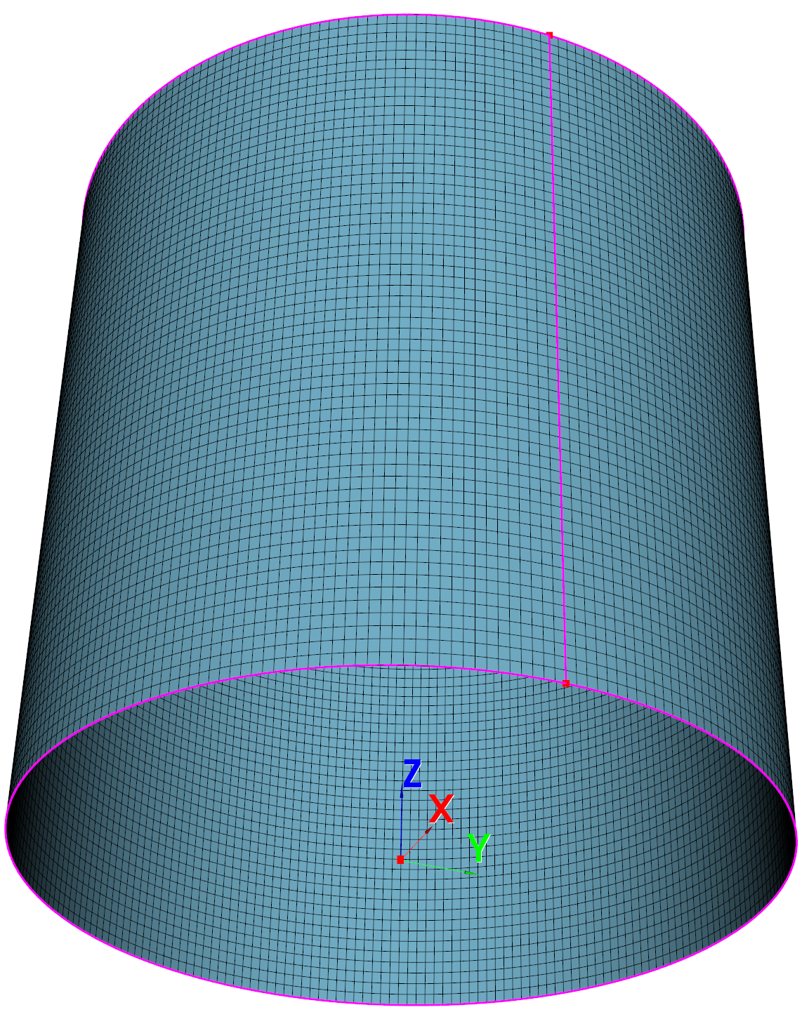
Cylinder model: Magenta: Edges. Red: Points.