3. Buckling Analysis

3.1. Collapse Analysis of Cylinder with Cutout

Folder: $B2EXAMPLES/buckling/cylinder_cutout

A cylinder with two opposite square cutouts is clamped at one end and compressed at the other end in the axial direction by an imposed displacement of 0.00425. This problem has been proposed by Almroth and Holmes [almroth1972] and has later been taken up by Knight and Rankin [knight2006]. The goal of this example is to demonstrate the collapse analysis and the post-processing capabilities of B2000++. Note that the B2000++ Verification Manual treats this case, too, but with Q4 and Q9 elements.

Similarly to Knight and Rankin, the problem is modeled with an eight of a cylinder (half in the longitudinal direction and a fourth in the circumferential direction):

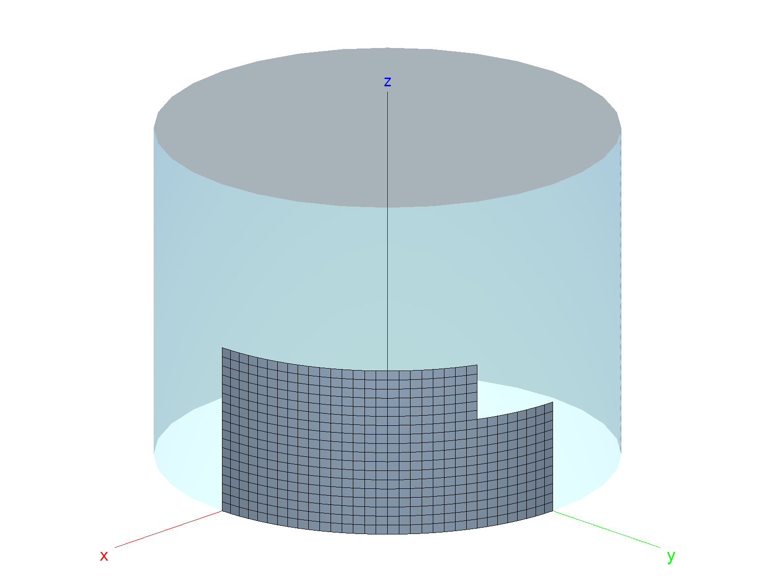
Cylinder with square cutouts: Mesh. 1/8 of cylinder is modeled.

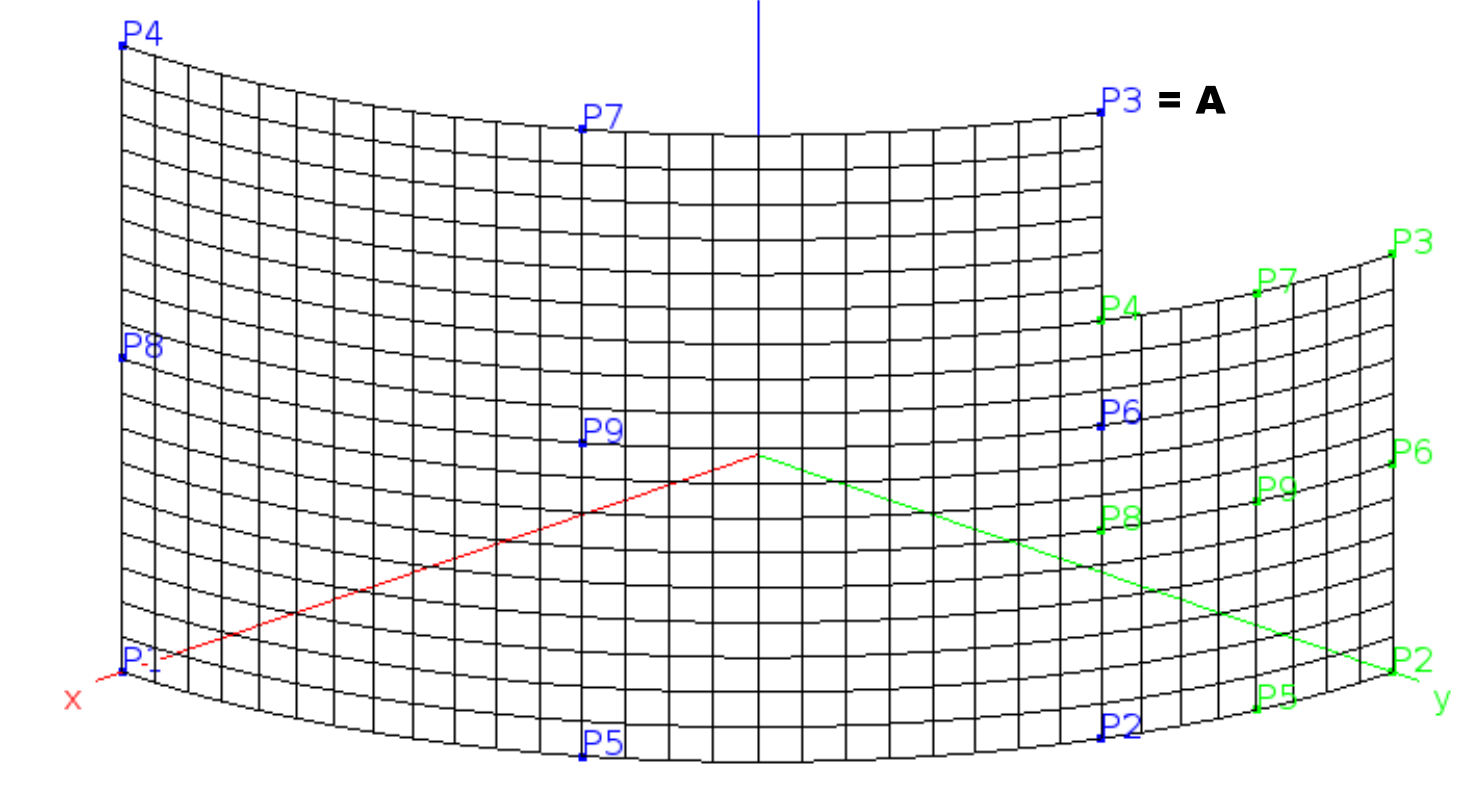
To this end, 2 cylindrical epatch patches are defined. The figure below displays the mesh with Q4.S.MITC elements. Boundary conditions are symmetry along both longitudinal edges (edges defined by blue points P1-P4 and green points P2-P3) and along one circumferential edge (edges defined by blue points P3-P4), the other circumferential edge being clamped.

EPATCHes and mesh.

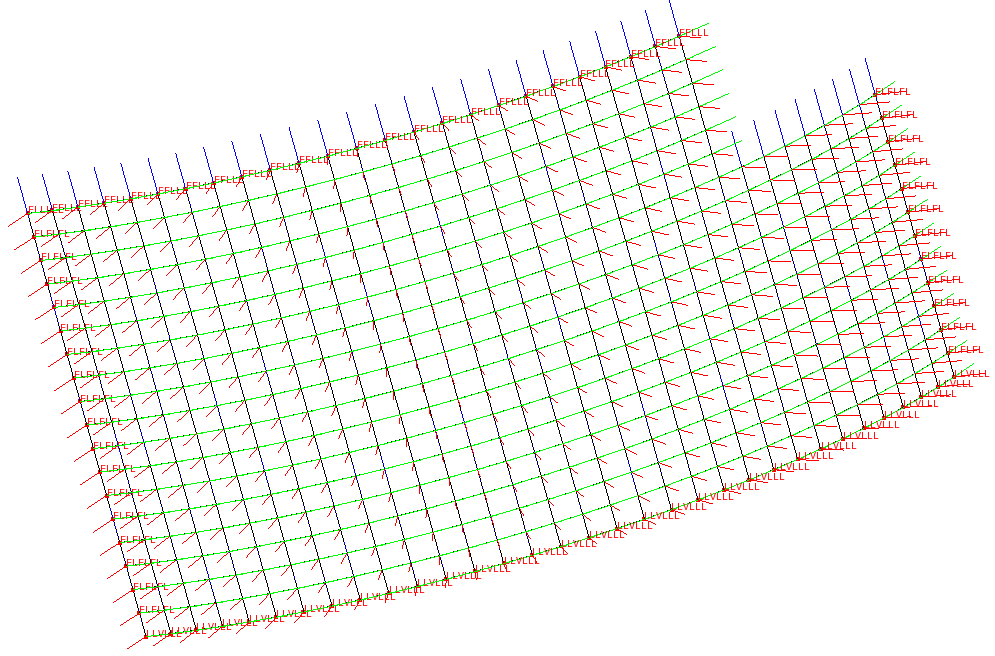
Boundary conditions and local node coordinate systems.

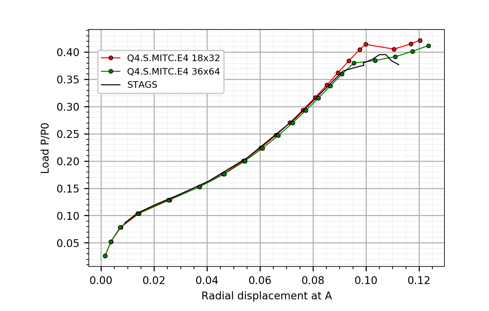
The test is run with Q4.S.MITC.E4 shell elements, comparing the cutout tip displacement-load function (point A) against the reported solution by Knight and Rankin.

The analysis control block contains a standard set of options, the non-linear analysis method being the default continuation method):

case 1
   analysis nonlinear
   ebc 1
   ebc 2
   step_size_init 0.05
   step_size_max 0.05
   gradients 1
   rcfo_restrict nodeset "EndShortening"
end

The maximum step size limitation is imposed in order to obtain a load curve with some points. Note the rcfo_restrict option: It contains the node set(s) containing all nodes involved in the imposed displacement, thus rendering post-processing very easy (see stroke-load diagram below).

The y-axis of both diagrams below are scaled to the reaction force \(P/P_{0}\), with \(P_{0} = {{1.2}\pi Et^{2}}\), where \(E=1 \times 10^{7}\) and \(t=0.014\).

The Simples script run.py (1) runs the analysis for selected mesh densities, extracting the graphs for each analysis and (2) collects the graphs and produces the stroke versus load disp_load.png and stroke_load.png out of plane versus load plots.

# Python script for executing a series of B2000++ runs with increasing
# mesh density for different element types, followed by a synthesis
# graph.

import os

import simples as si

# Comparison values obtained with STAGS
stags_dx = [0.00891496, 0.0137947, 0.0204575, 0.0290596, 0.0404457,
            0.0551476, 0.0731026, 0.0914018, 0.0975327, 0.0991906, 0.0989717,
            0.102444, 0.105009, 0.107511, 0.109607, 0.112328]
stags_load = [0.086217, 0.104633, 0.119883, 0.137595, 0.162698,
              0.205865, 0.277067, 0.365396, 0.373607, 0.375367,
              0.379707, 0.386628, 0.394956, 0.395191, 0.38393,
              0.376657]

os.system("rm -rf *.b2m *.modeler")

# Compute P0 = Analytical buckling load of cylinder
E = 1e7
t = 0.014
P0 = 0.25*1.2*3.14159*E*t**2

# Run analysis for different mesh densities for one element type
eltype = 'Q4.S.MITC.E4'
radial_disp_reaction_graphs = []
stroke_reaction_graphs = []
meshes = ((18,32), (36,64))
for ne in meshes:
    mesd = '%s %dx%d' % (eltype, ne[0], ne[1])
    print('Run for mesh density %s' % mesd)
    # Run B2000++ for current parameters
    if si.util.solve('cutout.mdl', params={'ELTYPE': eltype, 'NE1': ne[0], 'NE2': ne[1]}):

        # Open db and get node id of point A.
        model = si.Model('cutout.b2m', 'or')

        # Get internal node number of epatch 1 point P3 == point A.
        point = model.get_node_set('EPATCH-1-P')[2]

        # Get all analysis steps values. Scale because TIME goes from
        # 0 to 1, but displacement constrains from 0 to 0.1
        steps = model.get_steps(scale = 0.1)

        # Get the displacements of node *point*. Extract the
        # node-local component 'radial', which is dof 1.
        dy = model.get_dof_value_of_steps('displacements', node = point, dof = 1, system = 'nl')

        # Get sum of all reaction forces due to displacement loading and scale.
        ry = model.get_reaction_force_of_steps(scale = 1./P0)

        model.close()

        # Create Graph for current model and add to list
        radial_disp_reaction_graphs.append((mesd, (dy, ry)))
        stroke_reaction_graphs.append((mesd, (steps, ry)))

# Plot all unctions
colors = ('red', 'green', 'blue', 'cyan', 'magenta', 'yellow')
markerw = 0.5
markers = 3.

g = si.Graph2()
for i, a in enumerate(radial_disp_reaction_graphs):
    xy = a[1]
    line = g.add_line(xy[0], xy[1])
    line.marker= 'o'
    line.markeredgewidth = markerw
    line.markersize = markers
    line.markerfacecolor = None
    line.color = colors[i]
    line.label = a[0]
line = g.add_line(stags_dx, stags_load)
line.color = 'black'
line.label = 'STAGS'
g.axes_label_x = 'Radial displacement at A'
g.axes_label_y = 'Load P/P0'
g.add_legend((.2, .7))
g.save('disp_load.png')

g = si.Graph2()
for i, a in enumerate(stroke_reaction_graphs):
    xy = a[1]
    line = g.add_line(xy[0], xy[1])
    line.marker= 'o'
    line.markeredgewidth = markerw
    line.markersize = markers
    line.markerfacecolor = None
    line.color = colors[i]
    line.label = a[0]
g.axes_label_x = 'Stroke'
g.axes_label_y = 'Load P/P0'
g.add_legend((.2, .7))
g.save('stroke_load.png')

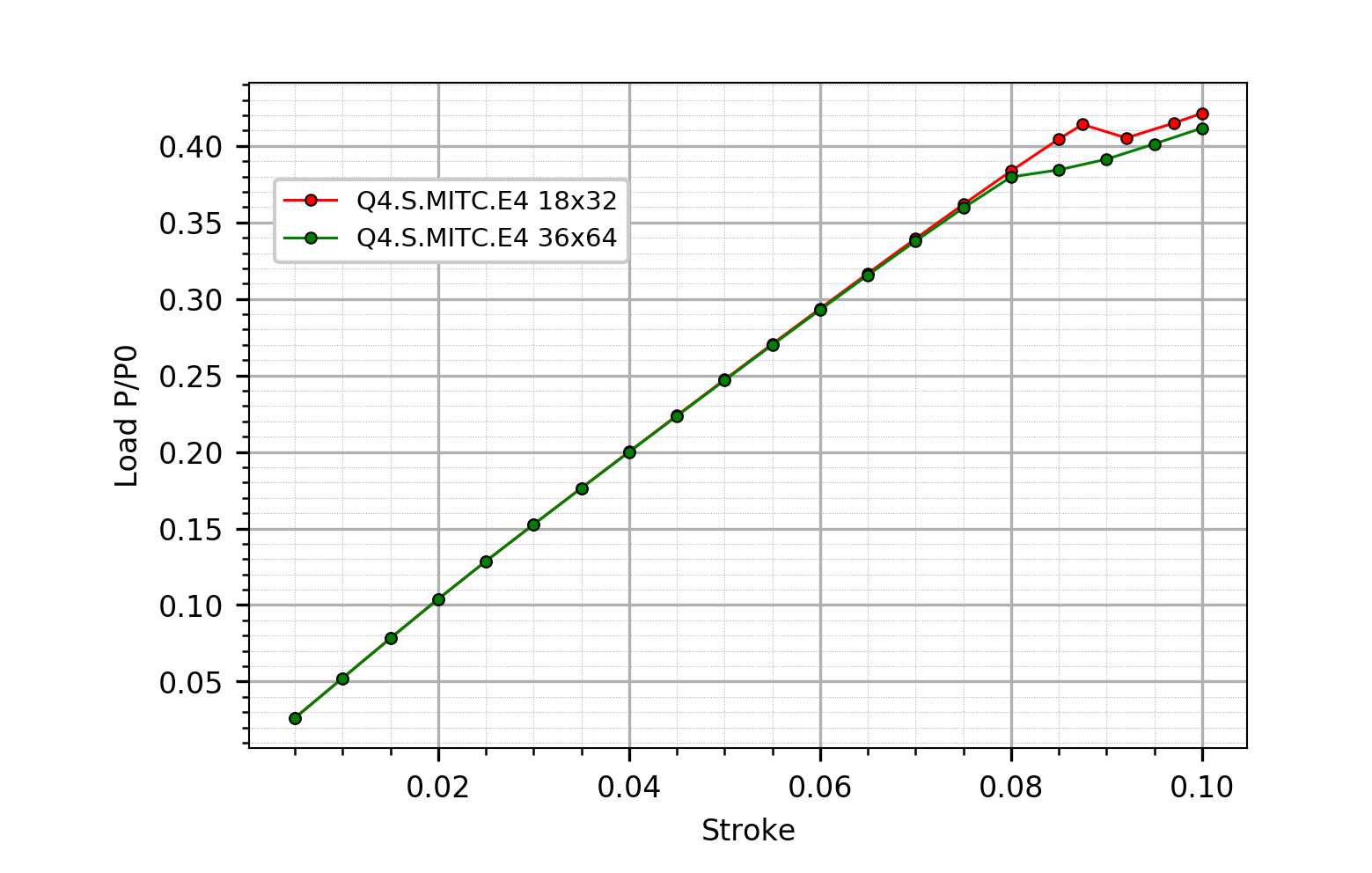
Stroke versus load diagram (Q4 mesh).

Out-of-plane versus load diagram (Q4 mesh).

3.2. Buckling of Three Stringer Composite Panel

Location of example: $B2EXAMPLES/buckling/panel3

The three string composite panel is a test case for demonstrating the B2000++ capabilities of dealing with lightweight composite structures modeled with shell or solid elements. A cylindrical panel with 3 stiffeners is subjected to axial compression load. The lowest buckling loads are to be determined.

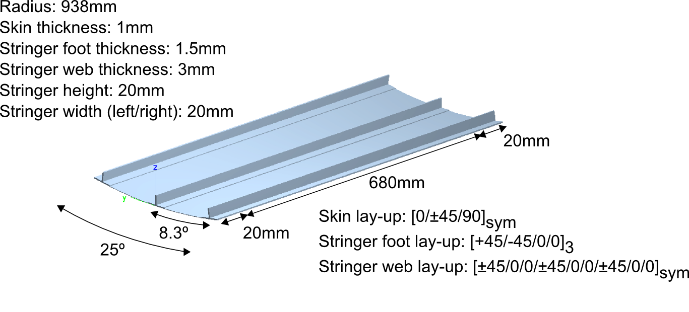
Three Stringer Composite Panel: Dimensions and laminate setup.

The boundary conditions are displayed in the figure below: Both curved edges are clamped and both straight edges are free. One of the curved edges is pushed towards the panel, causing it to buckle. All boundary conditions are essential boundary conditions (ebc command in the MDL input files) Thus, the resulting reaction force due to the edge displacement in axial direction is equal to the buckling load when multiplied by the computed eigenvalue.

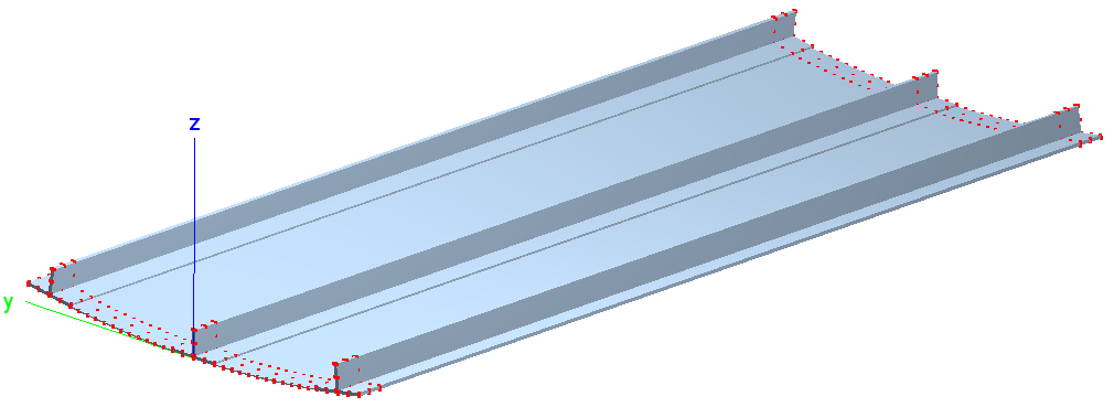
Three Stringer Composite Panel: Boundary conditions at nodes (red dots).

The shell model consists of Q9 MITC shell elements. The cylindrical shell and the shell plus the stringer foot are modeled with one element through the thickness, as is the stringer. The laminate orientations and laminate placement are visualized with baspl++:

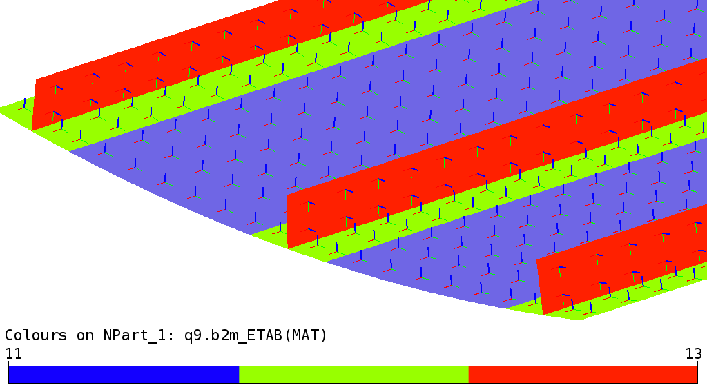
Three Stringer Composite Panel (solid model) : Laminates and material axis x (red) and y (green). Laminate 1 is material 11 (blue), laminate 2 is material 12 (yellow), and laminate 3 is material 13 (white).

Buckling modes without prestress of the shell model are computed for load case 1, requiring the first 10 modes:

case 1
  ebc       1
  analysis  linearised_prebuckling
  nmodes    10
  gradients 1
end

The buckling analysis is launched by the shell command

prompt> b2000++ --adir 'cases=1' -l "info of solver in cerr" shell.mdl

Linear buckling analysis results can be extracted and printed with b2print_buckling_loads:

b2print_buckling_loads shell

Linear reaction forces +2.9477108e+05

Number of computed buckling modes for case 1: 10
Mode Load factor    Critical force
   1 +1.7227278e-01 +5.0781032e+04
   2 +1.7237261e-01 +5.0810459e+04
   3 +1.7464288e-01 +5.1479669e+04
   4 +1.7469178e-01 +5.1494083e+04
   5 +1.7908786e-01 +5.2789922e+04
   6 +1.7965825e-01 +5.2958056e+04
   7 +1.8222893e-01 +5.3715819e+04
   8 +1.8233669e-01 +5.3747582e+04
   9 +1.8770931e-01 +5.5331277e+04
  10 +1.8883024e-01 +5.5661694e+04

The first buckling mode shape plot is obtained with the baspl++ script view_buckling_modes.py.

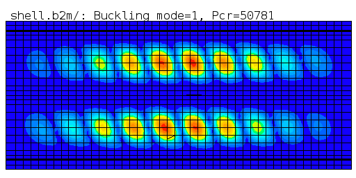
Three Stringer Composite Panel (shell model): First buckling mode.

3.3. Buckling of Composite Plate

Location of example: $B2EXAMPLES/buckling/plate

A simply-supported thin quadratic laminated plate of 500 mm by 500 mm is loaded with a forced displacement along one of the plate edges. The linearized buckling load as well as the post-buckling response due to the forced displacement of the edge is to be determined.

The plate is simply supported on all four edges, one edge being free to move in the x-direction to allow for the forced displacement. The plate is loaded with a forced displacement loading condition along the free edge 2.

Geometry and loading of plate

The plate is made of a composite material, 16 layers of 0.125mm thickness, with the symmetric stacking sequence (in degrees) \((+45,0,-45,0,+4,0,-45,+90)_s\). The material data are listed below:

\(E_1 = 146.86\ 10^{3} N/mm^2\)

\(E_2 = E_3 = 9.65\ 10\ 10^{3} N/mm^2\)

\(\nu_232 = \nu_13 = 0.023\)

\(G_12 = G_23 = G_13 = 45.5\ 10^{2} N/mm^2\)

FE Model

Now we explain in detail how to get to the solution. We start by defining the Finite Element model with the B2000++ model description language (MDL). MDL contains simple mesh generation capabilities with element patches. A single epatch defines the regular plate mesh and links to the material.

(et="Q4.S.MITC.E4")
(ne=40)

# Mesh definition
epatch 1
  geometry plate  # Geometry type
  p1 0.   0.   0. # 4 plate vertices
  p2 500. 0.   0.
  p3 500. 500. 0.
  p4 0.   500. 0.
  eltype (et)     # Element type
  ne1 (ne)        # N. of elements in first direction
  ne2 (ne)        # N. of elements in second direction
  mid 2           # Link to material identifier
end

Note the parametrization of the element type and the number of elements. Here we select Q4 four node quadrilateral MITC elements.

The plate geometry is uniquely defined by the four corner points p1, p2, p3, and p4 specified counter-clockwise, defining a flat plate. Note that the plate thickness is not needed if the material is a laminate material.

A laminate is defined with the MDL material block, by listing all layers one after the other, each layer specifying the thickness, the layer orientation, and the material identifier.

# Composite stacking sequence definition
material 2
  type laminate
  0.125  45 1
  0.125   0 1
  ...
end

For our model the default global material orientation is selected, i.e the material angle is defined with respect to the global coordinate system as displayed in the figure above.

The composite material constants are defined with a MDL material block, specifying the orthotropic material type.

material 1
  type orthotropic
  e1 146.86e+03
  e2 9.65e+03
  e3 9.65e+03
  nu12 0.3
  nu13 0.3
  nu23 0.023
  g1 45.5e+02
  g2 45.5e+02
  g3 45.5e+02
  failure max_principal_strain
    t +4500.e-6 # tension, micro-strain
    c -3000.e-6 # compression, micro-strain
    s +5000.e-6 # shear, micro-strain
    filter max_of_element
  end
end

A simple failure criterion is used, based on the maximum of the principal eigenvalues of the strain tensor. Its purpose is to select, for each element, the material point which is the most critical. This way, the amount of gradient data that is written to the database is reduced, which is important when working with laminate materials.

B2000++ discerns between essential boundary conditions (here: displacement constraints) and natural boundary conditions (here: forces). For our model we have to define the essential boundary conditions for (1) creating the required displacement constraints along edge 2 in the x-direction and (2) properly locking the structure along the edges.

Essential boundary conditions ebc along patch edges, i.e displacement constraints, can be added by referencing the proper epatch element (here: edge e2). MDL automatically generates the mesh node and element lists. They are stored on the model database and can be referenced by ebc and nbc boundary condition definitions.

The first ebc block 1 locks the structure. Since the edges are free to rotate we only lock the displacement DOFs, i.e DOFs UX, UY, or UZ::

ebc 1
   # Zero-value constraints
   value  0. dof [  UY UZ] epatch 1 e1  epatch 1 e2  epatch 1 e3   epatch 1 e4
   value  0. dof [UX     ] epatch 1 e4
end

The first line of the ebc block locks the y- and z-displacement DOFs of all edge nodes. The second line locks the x-displacement DOFs of the edge opposite to the moving edge (e2).

The second ebc block 2 applies a value for the x-displacement of all nodes of the edge e2:

ebc 2
   # Forced displacement
   value -1. dof  UX epatch 1 e2
end

The links to the ebc sets will be added to the case block, as will be described later.

For the particular configuration, i.e. a flat plate, an ‘imperfection’ has to be defined to trigger the post-buckling behavior. This can be achieved by defining a small out-ouf-plane force that ‘pushes’ the plate in the desired post-buckling direction (in the present model only one configuration is possible). The out-ouf-plane concentrated force of 1 N is assigned to the shell patch center node (identified with the epatch node p9) with a nbc block:

# Central out-of-plane force to create imperfection
nbc
  set 1
    value 1. dof FZ epatch 1 p9
  end
end

Note that, if node-local coordinates systems are defined (this is typically the case for curved shells), boundary conditions are defined with respect to the local coordinate system of the nodes associated to the DOF. In this example, however, there are no node-local coordinate systems. Hence, all boundary conditions are expressed in the global coordinate system.

All parameters related to an analysis case description are contained in a case block. In out example we will carry out 2 types of analysis, a buckling analysis and a post-buckling analysis.

Create model database

b2ip++ plate.mdl

Buckling Analysis

The case block for the buckling analysis defines the type of analysis, includes the links to the boundary conditions, and, for the buckling analysis type, defines the number of buckling modes to be computed.

case 1
  analysis  linearised_prebuckling
  nmodes    10
  ebc       1
  ebc       2
  gradients 1
end

adir
  # needs at least one case for -adir cases= to work
  case 1
end

In the analysis case description above, the buckling solver is activated for 10 buckling modes (note that selecting only a very small number buckling modes, such as 1 or 2, might lead to numerical problems in the eigensolver). The clamping and the displacement boundary conditions (ebc 1 and ebc 2) are activated.

The buckling analysis (case 1) is carried out by entering the shell command

prompt> b2000++ -adir cases=1  plate.b2m

After the analysis has completed, the b2print_buckling_loads prints the critical loads:

b2print_buckling_loads buckling

Eigenvalues and buckling loads, case 1
Contributing EBC identifiers: 2
Total reaction force F=(-158593, 2.50111e-12, -3.66168e-15)
amplitude Famp=158593

        Mode       Lambda   Crit. load
           1      0.01718         2725  *
           2      0.03948         6262  *
           3      0.05028         7973  *
           4      0.06912    1.096e+04  *
           5      0.08614    1.366e+04  *
           6       0.1099    1.743e+04  *
           7       0.1128    1.789e+04  *
           8       0.1335    2.117e+04  *
           9       0.1628    2.582e+04  *
          10       0.1632    2.588e+04  *

Lambda (eigenvalue): if > 1 no buckling, < 1 buckling, marked by *
Critical load: F * Lambda (if F != 0)
Reaction force: Sum of reactions due to EBC and NBC

Results can also be viewed with the b2browser. Enter the shell command below and click on “Solutions”, “case 1”, and “Buckling Loads”:

prompt> b2browser buckling

The buckling modes can be plotted with the baspl++ viewer. Enter the following shell command which displays the plate with the first buckling mode:

prompt> baspl++ plot_buckling_mode.py

The following image shows the shapes of some buckling modes:

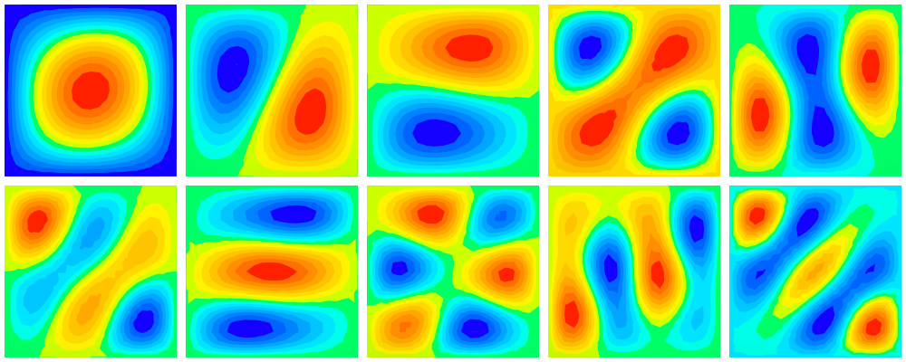
Buckling modes (amplitude plotted).

Post-Buckling Analysis

The case block for the post-buckling analysis case 2 defines the type of analysis, includes the links to the boundary conditions, and, for the buckling analysis type, defines the number of buckling modes to be computed.

case 2
   analysis        nonlinear
   ebc             1
   ebc             2 sfactor 0.1  # up to 0.1mm edge shortening
   nbc             1 sfunction 1. # constant force, not scaled by load factor
   step_size_init  0.01           # to get smoooth pre-buckling path
   step_size_max   0.01           # to get smoooth post-buckling path
   gradients       1              # compute gradients for all increments
   rcfo_restrict epatch 1 e2      # Restrict computation of reaction forces
                                  # to edge e2 nodes
end

The following comments pertain to the the post-buckling analysis case description above:

• The ebc 2 link includes the sfactor 0.1, which means that the load is incremented up to 0.1 times the ebc 2 values.

• The nbc 1 link includes sfunction 1.0, which means that the load of nbc 1 is applied constant during all increments.

• Setting step_size_init and step_size_max both to 0.01 , i.e. keeping the increments constant, will produce a smooth post-buckling path for the graphs, at the expense of higher computation time.2

• The rcfo_restrict option tells any post-processing tool, such as Simples, to restrict the computation of reaction forces to the nodes of the list (here: the epatch edge e2 nodes).

Post-buckling analysis is carried out by entering the shell command

prompt> b2000++ -adir cases=2 plate.b2m

INFO:solver.static_nonlinear:18:22:45.812: Start static nonlinear solver for case 1
INFO:solver:18:22:45.813: Resolving linear constraints: 102 equations.
INFO:solver:18:22:45.813: 0 dependent constraints were eliminated.
INFO:solver:18:22:45.813: Reduction matrix (903 x 1005) has 903 nonzeros.
INFO:solver.static_nonlinear:18:22:45.813: Start increment 1 of stage 1 for time 0 and time step 0.01.
INFO:solver.static_nonlinear:18:22:45.885: Start increment 2 of stage 1 for time 0.01 and time step 0.01.
...
INFO:solver.static_nonlinear:18:22:48.304: Start increment 99 of stage 1 for time 0.98 and time step 0.01.
INFO:solver.static_nonlinear:18:22:48.331: Start increment 100 of stage 1 for time 0.99 and time step 0.01.
INFO:solver.static_nonlinear:18:22:48.363: End static nonlinear analysis for case 1 with success.

After the analysis has completed, the simples script plot_postbuckling_graphs.py

prompt> python plot_post-buckling_graphs.py

plots the graphs below:

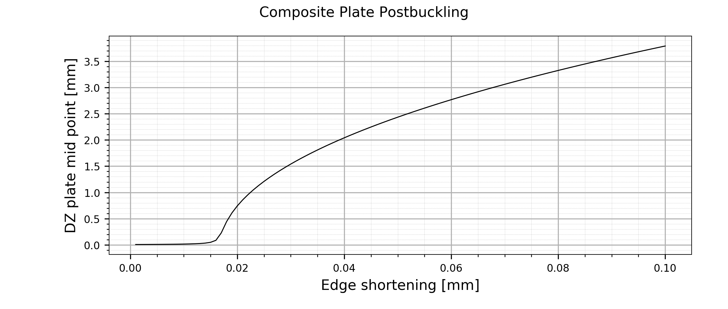
Mid-point out-of-plane displacement vs. edge shortening plot.

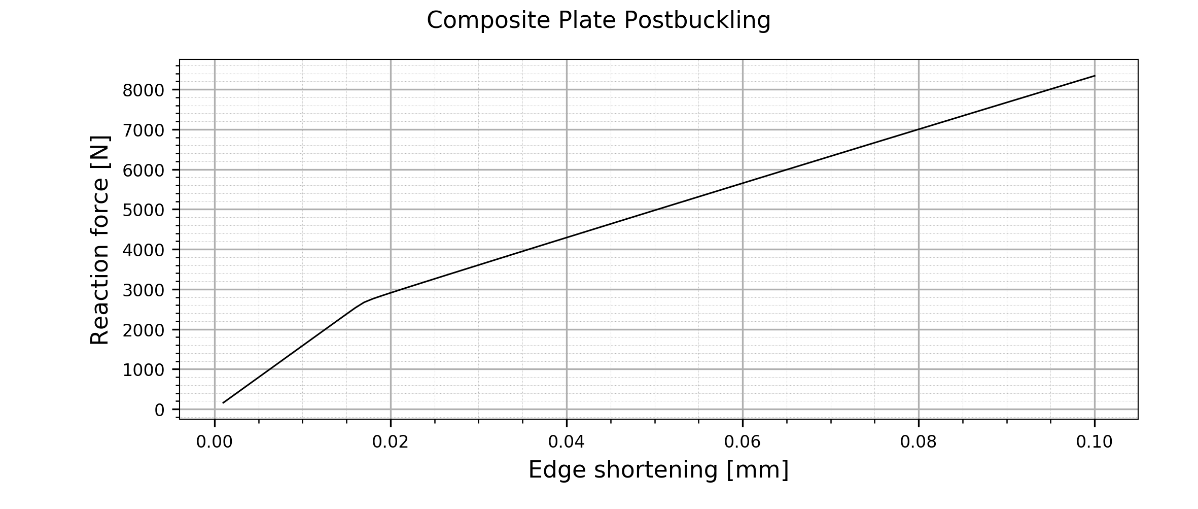
Total reaction force vs. edge shortening plot. The reaction force is the sum of all reaction forces applied to epatch edge e3.

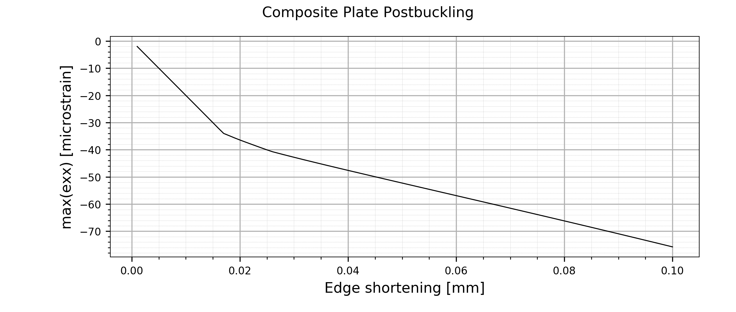
Maximum \(\epsilon_{xx}\) vs. edge shortening plot.

3.4. Restart of Curved Panel

Location of example: $B2EXAMPLES/buckling/restart

The test case computes the post-buckling behavior of a slightly curved panel, thereby testing the restart capabilities of B2000++.

The panel has a length L=92mm along the straight edges, a radius R=586mm with an angle α=9.0 degrees along the curved edges and a thickness t=1mm. The material is linear isotropic, with modulus of elasticity E=70000 Pa and Poisson number 0.3. The edge loads act on edge I in the positive z-direction. Displacements in radial direction on edge I are suppressed and edge IV is simply supported. Edge II and III have symmetric boundary conditions. The mesh density is 6 by 6 Q4 elements.

Due to symmetry, only one quarter of the panel is considered. The panel is modeled with Q4.S.MITC.E4 shell elements.

Slightly curved panel: Geometry

A first run is made with loading the panel to a load factor (time) of 1.0. With the last converged step (cycle) corresponding to load factor 1.0, a restart is made to a load factor (time) of 2.0.

Slightly curved panel: Displacement Uz of patch point P1 as a function of the load step (time). Red: Complete solution up to the load factor (time) of 2.0. Dots: Initial run up to the load factor (time) of 1.0.

The restart information is added to the database with the restart function (see file restart.py):

def restart(db, case=1, step=None, sfactor=2.0):
    """Modifies the database for an imminent restart from implicitly
    assumed last step (step=None) or from specified step (cycle).

    :param db db: pymemcom database object.

    :param int case: Case identifier.

    param int step: Step (cycle) from which to start analysis
    again. Default is last step found.

    :param foar sfactor: New sfactor to e reached at last step.

    """

    stage = 1 # first stage of case 1
    if not step:
        laststep = db[f'SOLUTION-STAGE.0.0.0.{case}.{stage}'][:]['LAST_STEP'][0]
    else:
        laststep = step

    # print(f'Restart from last step={laststep}, time={time}')
    db[f'CASE.{case}'][0]['SFACTOR']=sfactor
    db[f'CASE.{case}'].desc['DOF_INIT']=f'DISP.*.{laststep}.0.{case}'
    db[f'CASE.{case}'].desc['STEP_INIT_NUM']=laststep
    # time = db[f'SOLUTION-STEP.0.{laststep}.0.1'][:]['TIME'][0]
    # db[f'CASE.{case}'].desc['TIME']=time
    db.close()

3.5. Rod Snap Problem

Location of verification case: $B2EXAMPLES/buckling/snap

This simple problem consisting of two rods illustrates the snap phenomenon and its solution with B2000++. Note that this model is purely theoretical, because the material is assumed linear elastic!

The FE model is shown below, the rods being inclined by 10 degrees. Material is linear isotropic with a modulus of elasticity roughly corresponding to neoprene or similar. The geometric and material values can be consulted in file rod.mdl.

The model is constrained at nodes 1 and 3, node 2 being free to move in the x- and y-direction. A load (nbc) \(F_y=-200\) is applied at node 2.

Rod snap problem: FE model, load, and constraints.

When trying to solve the problem for the natural boundary condition case, i.e the case with a force \(F_y\) applied in the y-direction of node 2, the Newton-type solution procedure will fail, because the procedure will not overcome the situation where \(U_y=H\). Arch-length methods are then indicated (see input files).

The applied load \(F_y\) (figure above) of load case 1 is increased up to a factor 10. Since we do not increment from 0 to 1 we need to define at least one stage.

Two models are compared:

• A model with 1 stage with a SFACTOR of 10 (1stage.mdl). The case 1 block then adds a single stage (i.e case) 11, defining the constraint (ebc) set, the load (nbc) set, and the single stage 11:

  case 1
    analysis               nonlinear
    increment_control_type hyperplane
    stage                  11 sfactor 10.0
    gradients 1
  end
  

• A model with 2 stages, each with a SFACTOR of 5, leading to a final SFACTOR of 10 (2stages.mdl). Observe that, with the selected step increment parameters, the solution jumps to secondary branch! The case 1 block then adds 2 stages (i.e case) 11 and 12, defining the constraint (ebc) set, the load (nbc) set, and the stages 11 and 12:

  case 1
    analysis nonlinear
    increment_control_type hyperplane
    stage 11 sfactor 5
    stage 12 sfactor 5
    gradients 1
  end
  

Rod snap problem: Compare solutions obtained with 1 stage or with 2 stages: Displacement \(U_y\) plotted against the load scale factor SFACTOR.

Rod snap problem: Displacement \(U_y\) and rod stress plotted against the load scale factor SFACTOR (1 stage).