2. Static Analysis
2.1. Cable Truss
Folder: $B2EXAMPLES/static/cable_truss
A truss composed of prestressed cables deforms under its own weight
(simulated here by forces concentrated at the truss free nodes) and
under an additional single force applied at one node. The model has
been presented by Kar et.al [kar] . The non-linear analysis can be
executed in one or in several stages being executed one after the
other in the order they are enumerated in the case
definition. Each stage references a case specifying sets of boundary
conditions and analysis parameters and the solution will be
incremented to a load or time parameter of 1.0 unless specified
otherwise by the sfactor option of the stage.
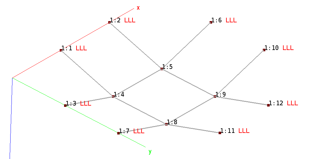
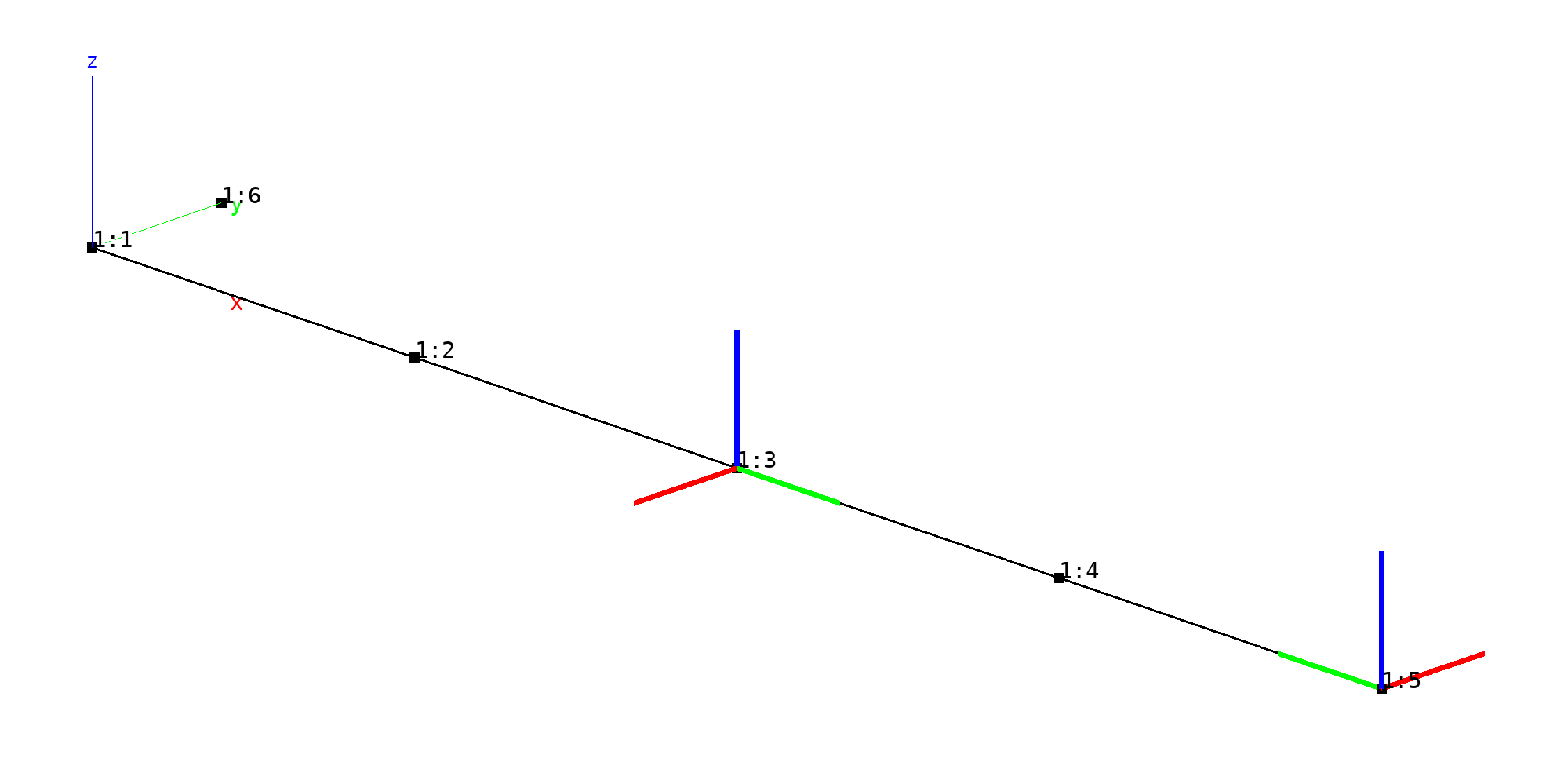
Cable truss mesh. Nodes are marked branch:node, where branch is the
branch identifier and node the external node identifier. Boundary
conditions (red) are marked LLL, i.e displacements locked in all 3
directions at nodes 1, 2, 3, 6, 7, 10, 11, 12).
Two different cases are presented, all three leading to the same result. The problem must be solved in 3 steps (see also note below):
Run the input processor b2ip++, defining all 3 cases (see input file
cable.mdl.Run for case 1 with the solver option
adir cases=1.Run for case 2 with the solver option
adir cases=2.
The database now contains the 3 runs and the load-stress curves can be extracted (see diagrams below).
Note
The non-linear B2000++ solver can treat more than one nonlinear case in a single model. However, the cases must be executed one by one.
Case 1: The analysis is performed in one stage, with all boundary
conditions (dead weight plus load) applied simultaneously. Case 1
tries to solve for all boundary conditions in one stage. Essential
boundary conditions are defined in set 1 (option ebc 1). Loads are
defined in natural boundary condition sets 1 and 2. The solver will
try to solve for the final default load scale factor of 1.0 (when no
stage is defined). Step control: In case the step size is too large,
steps can become smaller, but not less that 0.01 (option
step_size_min 0.01). :
case 1
    title 'Dead weight and useful loads in 1 set'
    analysis nonlinear
    ebc 1  # Zero constraints
    nbc 1  # Dead weight
    nbc 2  # Useful load
    step_size_init 0.1
    step_size_min 0.01
    step_size_max 0.1
    gradients 1
end
The output from B2000++ is listed below (it is obtained with the
B2000+ command option -l):
b2000++ -l 'info of all in err' -adir 'cases=1' b2test.b2m
INFO:all:10:45:58.554: Start
INFO:solver.static_nonlinear:10:45:58.555: Start static nonlinear solver for case 1
INFO:domain:10:45:58.555: Total number of DOfs: 36.
INFO:solver.static_nonlinear:10:45:58.556: Start prediction of increment 1 of stage id 1 for time 0.
INFO:solver.static_nonlinear:10:45:58.591: Start correction of increment 1 of stage id 1 for time 1.
INFO:solver.static_nonlinear:10:45:58.595: End static nonlinear analysis for case 1 with success.
INFO:all:10:45:58.595: End of execution
Case 2: Case 2 solves the stages 21 and 21 in the order they are
enumerated in the case 2 block. Again, essential boundary
conditions are defined in ebc set 1 (option ebc 1). The stage with
the dead weight, i.e case 21, refers to the natural boundary condition
set 21 (option nbc 21), which is solved up to the default load
scale factor 1.0. The solver then continues with the next stage,
i.e. case 22, which refers to the natural boundary condition set 22
(option nbc 22), solving for the final load multiplier value of
that stage, i.e. (default) 1.0.
22):
case 2
    title 'Stage 1 (own weight) and stage 2 (useful load)'
    analysis nonlinear
    stage 21 sfactor 1  # Dead weight
    stage 22 sfactor 1  # Useful load
    gradients 1
end

stage 21
    title 'Stage 1 (first stage, dead weight)'
    ebc 1  # Zero constraints
    nbc 1  # Dead weight
    step_size_init 0.1
    step_size_min 0.01
    step_size_max 0.1
end

stage 22
    title 'Stage 2 (useful load)'
    nbc 2  # Useful load added to all nbc's
    step_size_init 0.1
    step_size_min 0.01
    step_size_max 0.1
end
Both cases give the same result for the final load factor, although the path to the solution is not the same, i.e it depends on the load stages. Note that case 2 goes to a final load factor of 2 because of the 2 stages, while cases 1 and 2 go to the final load factor of 1.0.

Load case 1: Displacement and rod stress.

Load case 2: Displacement and rod stress. Note: The path is not the same as for case 1.
Deformations can be viewed with baspl++, the viewer script view.py
producing the deformation plot with the cable stresses shown below
for case 1. To run the viewer from the shell, type
baspl++ -t view.py
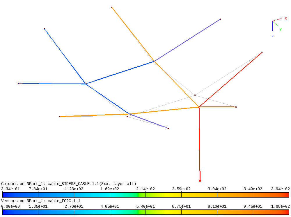
Deformed cable truss shape and cable stress (colored elements) and applied force.
In addition, node displacements of all cases can be printed with the B2000++ model browser b2browser.
b2browser cable
and click Solutions, Case 1, Displacements, Cycle 10 (the final cycle):
Displacements and Rotations (DISP), dataset "DISP.1.10.0.1", cycle=10, subcycle=0, case=1

      EID        UX           UY           UZ           RX           RY           RZ       Amplitude
        1 G           0            0            0            0
        2 G           0            0            0            0
        3 G           0            0            0            0
        4 G     -0.3509      -0.3509        0.887        1.016
        5 G     -0.5581        3.269       -2.816        4.351
        6 G           0            0            0            0
        7 G           0            0            0            0
        8 G       3.269      -0.5581       -2.816        4.351
        9 G       3.615        3.615        16.31        17.09
       10 G           0            0            0            0
       11 G           0            0            0            0
       12 G           0            0            0            0
Largest amplitude=17.0906
Absolute printout cutoff value threshold=1e-100
2.2. Cylinder with RBE/FMDE Elements
Folder: $B2EXAMPLES/static/cylinder_rbe
This example demonstrates RBE Elements; RBE (rigid body element) example and FMDE Elements; FMDE (Force-Moment Distribution Element) example elements for defining boundary conditions (constraints) applied to a a cylinder section Boundary conditions; Apply with RBE elements. The model is a cylinder clamped at one end \(z=0\) and loaded at the other end \(z=L\). To introduce the corresponding boundary conditions, RBE/FMDE elements are introduced:
The clamping condition is formulated with a RBE/FMDE element connecting all DOFs of a node at (0,0,0) to all circumferential nodes of the cylinder at \(z=0\). The constraints (ebc) will be applied to that node. The RBE element acts as a rigid diaphragm in the xy-plane.
The load condition is formulated with a RBE element connecting a node at (0,0,L) with all circumferential nodes of the cylinder at \(z=L\). The force (nbc) will be applied to that node. The RBE/FMDE element acts as a rigid diaphragm in the xy-plane.
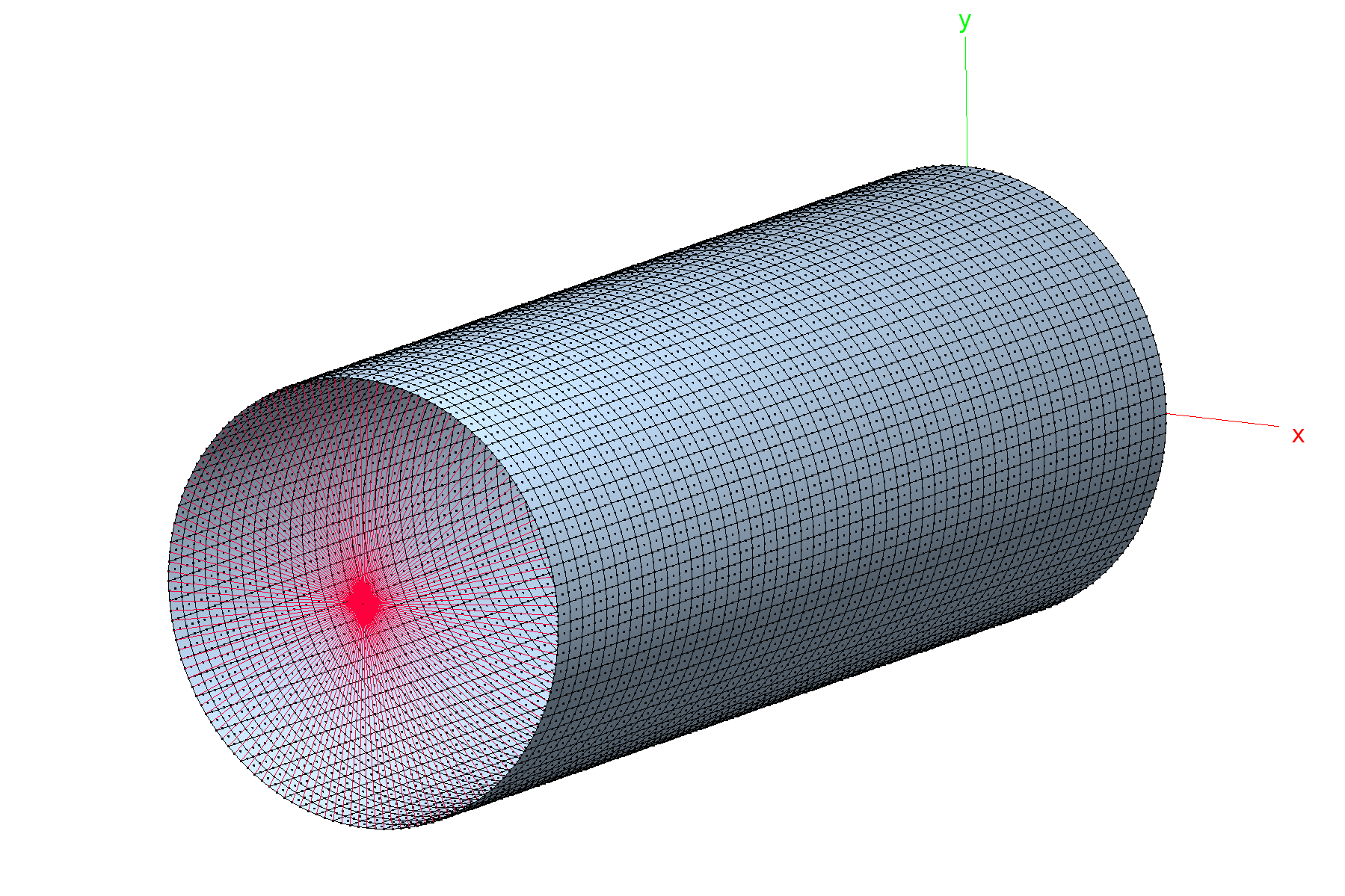
Cylinder FE mesh: Q9 shell element mesh (blue) and RBE/FMDE mesh (red).
Dimensions and material parameters of the cylinder model:
L = 1.0    # Length of cylinder [m]
R = 0.3    # Radius of cylinder [m]
T = 0.0005 # Thickness of cylinder [m]
Fx = 1.e5  # Axial load [N]
E = 72.4e9 # Young's modulus [N/m2]
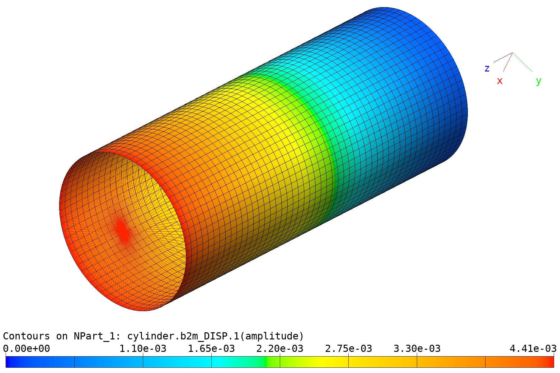
Cylinder model: Deformation amplitude, traction case.
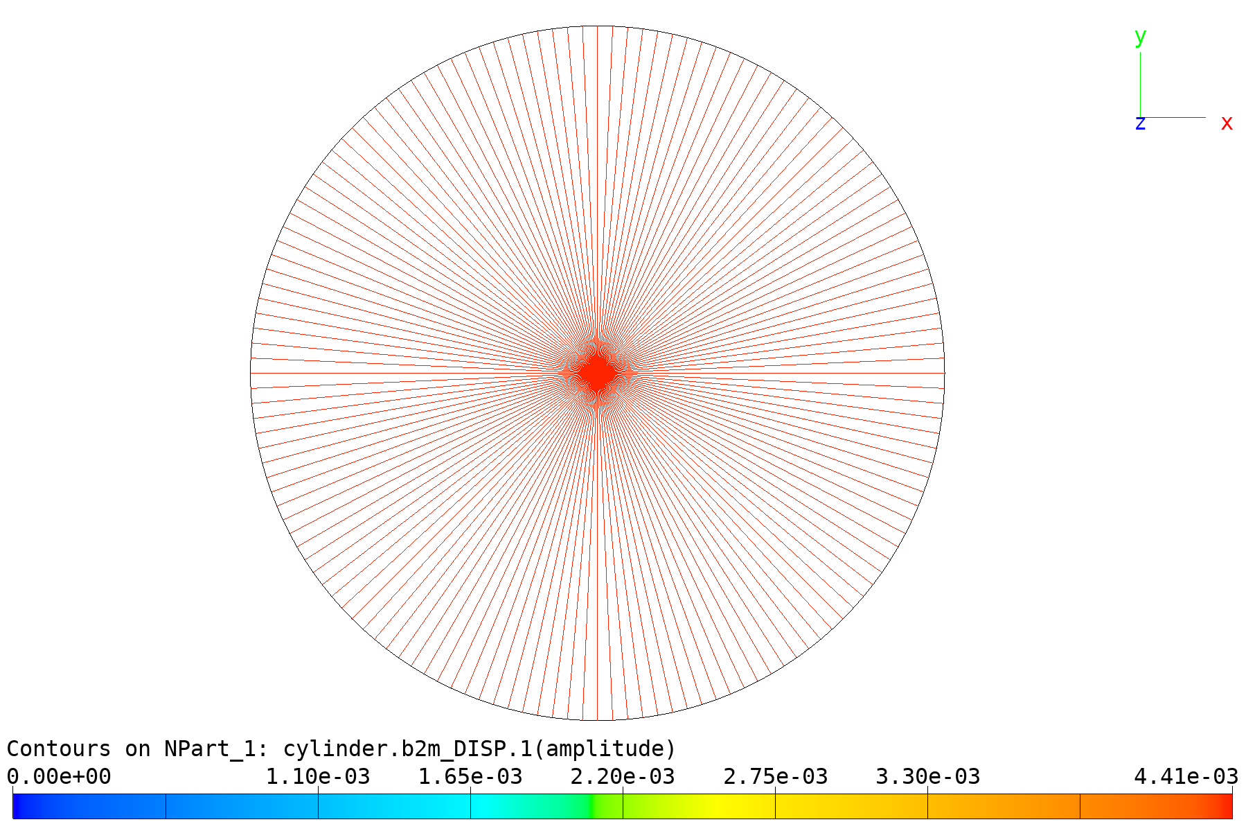
Cylinder model: Deformation amplitude of RBE/FMDE element, traction case.
2.3. Laminate Material (1 Element Test)
Folder: $B2EXAMPLES/static/laminate1
This one-element model consists of a rectangular four-node Q4 shell element in the global x-y plane The model is “statically determinate”, i.e the number of constrained degrees of freedom is equal to the number of rigid body movements, i.e 3 translations and 3 rotations. The plate is pulled in the element x-direction (fiber 1 direction, see figure below).
The purpose of this example is to
Demonstrate laminate material in shells with a one layer material with 0°, 90° fiber orientations, and with a four layer 0°/90°/90°/0° material.
Explain the basic concepts of coordinate systems.
Forces (natural boundary conditions) are added as point forces in order to illustrate the concept of node-local coordinate systems. The total force applied is selected such that the stress in fiber direction 1 becomes 500 MPa:
The first test 0.mdl defines a model in the branch-global
(=global-global) x-y plane:
The branch-global system is identical to the global-global system (no branch orientation specified).
The coordinates are formulated in the branch-global system.
The element local x-axis coincides with the branch-global x-axis.
The node-local directions of the degrees-of-freedom coincide with the branch-global direction.
The zero constraints (essential boundary conditions, ebc) do not need node-local transformations.
The applied forces \(F=0.5*F_{tot}\) in the branch-global x-direction do not need node-local transformations.

One-element laminate test: Element local x-axis coincides with branch-global x-axis. Gray: mesh, blue: deformed mesh, red: constrains, green: forces.
The second test 30.mdl defines a model in the branch-global
(=global-global) x-y plane with the element local x-axis rotated by
30° around the branch-global z-axis with respect to the
branch-global x-axis:
The branch-global system is identical to the global-global system (no branch orientation specified).
The coordinates are formulated in the branch-global system.
The orientation of the values at the mesh nodes (forces, constraint) are formulated in a node-local orientation system with the MDL transformation command
transformations
    1 cartesian 0 0 0  0 0 1  (cos30) (sin30) 0
end
and referred to by the
transformationparameter of the MDL nodes command:nodes transformation 1 1 0.0 0.0 0.0 2 7.53442101 4.35 0.0 3 6.38442101 6.34185843 0.0 4 -1.15 1.99185843 0.0 end
The zero constraints (essential boundary conditions, ebc) are formulated in the node-local system, because the nodes involved have a local transformation.
The applied forces \(F=0.5*F_{tot}\) are formulated in the node-local system, because the nodes involved have a local transformation.

One-element laminate test: Model rotated 30° around the branch-global z-axis. Gray: mesh, blue: deformed mesh, red: constrains, green: forces.
- The third test
30btrf.mdldefines a model in a branch-global transformed with respect to the global-global system by a branch_orientation command:
The branch-global system is rotated with the MDL branch_orientation command by 30° around the global-global z-axis:
branch_orientation
    rotate axis z angle 30
end
The coordinates are formulated in the branch-global system and are identical to the coordinates of model
0.mdl.The element local x-axis coincides with the branch-global x-axis.
The node-local directions of the degrees-of-freedom coincide with the branch-global direction (no node-local transformation).
The zero constraints (essential boundary conditions, ebc) do not need node-local transformations.
The applied forces \(F=0.5*F_{tot}\) in the branch-global x-direction do not need node-local transformations.
Comparison of the results of the three models (the solutions of the analysis) is discussed. To resume, please note that:
DOF fields, i.e. displacements and rotations, are stored on the B2000++ model database with respect to the branch-global coordinate system. Values at nodes with node-local coordinate systems (orientations) are transformed to the branch-global orientation.
Element stress and strain tensors as well as any other sampling point field values, i.e element-related derived quantities, are stored on the B2000++ model database with respect to the branch-global coordinate system.
Displacements of nodes 2 and 3 as stored on the B2000++ model database are compared in the table below:
   Model  EID           DX           DY    Amplitude
     "0"    2      0.02962            0      0.02962
            3      0.02962    -0.002349      0.02971

    "30"    2      0.02565      0.01481      0.02962
            3      0.02683      0.01278      0.02971

"30btrf"    2      0.02962            0      0.02962
            3      0.02962    -0.002349      0.02971
Displacements of model 0 and 30btrf are identical, because
both models are formulated in the same branch global configuration.
Stresses at specific points can be plotted or printed with the b2plot_stack script.
script. Example: Plot stresses through the shell thickness z' at Gauss integration point 1 of element 1.
b2plot_stack -item 1 -g 2 --case 1 -f STRESS 30.b2m

Model 30: Stresses through shell thickness z' at Gauss integration point 1 of element 1.
Print stresses through the shell thickness z' for all integration points (r,s,t coordinates) of element 1.
b2print_stack --items=1 30.b2m

STRESS, element 1, case=1, cycle=0
----------------------------------

 Layer        r        s         t        Sxx        Syy  Szz        Sxy  Syz  Sxz
     1 -0.57735 -0.57735 -1.000000 523.508998 183.351171  0.0 294.585320  0.0  0.0
     1  0.57735 -0.57735 -1.000000 523.508997 183.351171  0.0 294.585320  0.0 -0.0
     1 -0.57735  0.57735 -1.000000 523.508998 183.351171  0.0 294.585320  0.0  0.0
     1  0.57735  0.57735 -1.000000 523.508998 183.351171  0.0 294.585320  0.0 -0.0
     1 -0.57735 -0.57735 -0.666667 523.508998 183.351171  0.0 294.585320  0.0  0.0
     1  0.57735 -0.57735 -0.666667 523.508997 183.351171  0.0 294.585320  0.0 -0.0
     1 -0.57735  0.57735 -0.666667 523.508998 183.351171  0.0 294.585320  0.0  0.0
     1  0.57735  0.57735 -0.666667 523.508998 183.351171  0.0 294.585320  0.0 -0.0
     1 -0.57735 -0.57735 -0.333333 523.508998 183.351171  0.0 294.585320  0.0  0.0
     1  0.57735 -0.57735 -0.333333 523.508997 183.351171  0.0 294.585320  0.0 -0.0
     1 -0.57735  0.57735 -0.333333 523.508998 183.351171  0.0 294.585320  0.0  0.0
     1  0.57735  0.57735 -0.333333 523.508998 183.351171  0.0 294.585320  0.0 -0.0
     2 -0.57735 -0.57735 -0.111111  34.485860  -2.408982  0.0  31.951871  0.0  0.0
     2  0.57735 -0.57735 -0.111111  34.485860  -2.408982 -0.0  31.951871 -0.0  0.0
     2 -0.57735  0.57735 -0.111111  34.485860  -2.408982  0.0  31.951871  0.0  0.0
     2  0.57735  0.57735 -0.111111  34.485860  -2.408982 -0.0  31.951871 -0.0  0.0
     3 -0.57735 -0.57735  0.277778  34.485860  -2.408982  0.0  31.951871  0.0  0.0
     3  0.57735 -0.57735  0.277778  34.485860  -2.408982 -0.0  31.951871  0.0 -0.0
     3 -0.57735  0.57735  0.277778  34.485860  -2.408982  0.0  31.951871  0.0  0.0
     3  0.57735  0.57735  0.277778  34.485860  -2.408982 -0.0  31.951871  0.0 -0.0
     4 -0.57735 -0.57735  0.444444 523.508998 183.351171  0.0 294.585320  0.0  0.0
     4  0.57735 -0.57735  0.444444 523.508997 183.351171  0.0 294.585320 -0.0  0.0
     4 -0.57735  0.57735  0.444444 523.508998 183.351171  0.0 294.585320  0.0  0.0
     4  0.57735  0.57735  0.444444 523.508998 183.351171  0.0 294.585320 -0.0  0.0
     4 -0.57735 -0.57735  0.722222 523.508998 183.351171  0.0 294.585320  0.0  0.0
     4  0.57735 -0.57735  0.722222 523.508997 183.351171  0.0 294.585320 -0.0  0.0
     4 -0.57735  0.57735  0.722222 523.508998 183.351171  0.0 294.585320  0.0  0.0
     4  0.57735  0.57735  0.722222 523.508998 183.351171  0.0 294.585320 -0.0  0.0
     4 -0.57735 -0.57735  1.000000 523.508998 183.351171  0.0 294.585320  0.0  0.0
     4  0.57735 -0.57735  1.000000 523.508997 183.351171  0.0 294.585320 -0.0  0.0
     4 -0.57735  0.57735  1.000000 523.508998 183.351171  0.0 294.585320  0.0  0.0
     4  0.57735  0.57735  1.000000 523.508998 183.351171  0.0 294.585320 -0.0  0.0
2.4. Solid Elements Element Integration Demos
This one-element model demonstrates working with laminates in solid elements. Two models are generated: One with a single element and 4 layers and one with 4 elements through the z-direction.
one.mdl: Linear static solid mechanics test with one element and multiple layers. The MDL element parameter ischeme defines the integration scheme per layer:
ischeme GAUSS2x2x1will produce 4 integration points per layer andischeme GAUSS2x2x2will produce 8 integration points (2 through the layer).stacked.mdl: Linear static solid mechanics test with one layer per element and elements stacked. The complete stack has the same dimension in z as the one element model. Result should be very near the
one.mdltest. The MDL element parameter ischeme defines the integration scheme per element:ischeme GAUSS2x2x1will produce 4 integration points per element andischeme GAUSS2x2x2will produce 8 integration points (2 through the element z-direction).
Run the one element model with (example with ischeme GAUSS2x2x1,
producing 4 points per layer and 4 layers):
sh ./run.sh one

"DISP": Displacements and Rotations, mesh=1, case=1, cycle=0, selection="All nodes"

         EID           Ux           Uy           Uz
           1            0            0            0
           2    0.0001889   -1.495e-18   -1.873e-05
           3            0            0            0
           4    0.0001889   -1.505e-18   -1.873e-05
           5            0            0            0
           6    0.0001927   -1.528e-18   -1.873e-05
           7            0            0            0
           8    0.0001927   -1.536e-18   -1.873e-05

"STRESS": Cauchy/linear stress, global reference frame, mesh=1, case=1, cycle=0, selection="All elements"

    IDENT           IP            Sxx          Syy          Szz          Sxy          Syz           Sxz
        1            1 132568619.4183       0.0000       0.0000      -0.0000      -0.0000 -3784352.4404
        1            2 132568619.4183       0.0000       0.0000      -0.0000      -0.0000  3784352.4404
        1            3 132568619.4183       0.0000       0.0000      -0.0000      -0.0000 -3784352.4404
        1            4 132568619.4183       0.0000       0.0000      -0.0000      -0.0000  3784352.4404
        1            5 133224088.4883       0.0000       0.0000      -0.0000      -0.0000 -3784352.4404
        1            6 133224088.4883       0.0000       0.0000       0.0000      -0.0000  3784352.4404
        1            7 133224088.4883       0.0000       0.0000      -0.0000      -0.0000 -3784352.4404
        1            8 133224088.4883       0.0000       0.0000       0.0000      -0.0000  3784352.4404
        1            9  66939778.7792       0.0000       0.0000      -0.0000      -0.0000 -1892176.2202
        1           10  66939778.7792       0.0000       0.0000       0.0000      -0.0000  1892176.2202
        1           11  66939778.7792       0.0000       0.0000      -0.0000      -0.0000 -1892176.2202
        1           12  66939778.7792       0.0000       0.0000       0.0000      -0.0000  1892176.2202
        1           13  67267513.3142       0.0000       0.0000       0.0000      -0.0000 -1892176.2202
        1           14  67267513.3142       0.0000       0.0000       0.0000      -0.0000  1892176.2202
        1           15  67267513.3142       0.0000       0.0000       0.0000      -0.0000 -1892176.2202
        1           16  67267513.3142       0.0000       0.0000       0.0000      -0.0000  1892176.2202
Run the stacked elements model with (example with ischeme GAUSS2x2x2,
producing stresses for 4 elements with 2 by 2 by 2 integration points:
sh ./run.sh stacked

"DISP": Displacements and Rotations, mesh=1, case=1, cycle=0, selection="All nodes"

         EID           Ux           Uy           Uz
        1            0            0            0
        2     0.000189    6.154e-18   -1.868e-05
        3            0            0            0
        4     0.000189    6.155e-18   -1.868e-05
        5            0            0            0
        6    0.0001897    5.348e-18   -1.868e-05
        7            0            0            0
        8    0.0001897    5.349e-18   -1.868e-05
        9            0            0            0
       10    0.0001907    4.543e-18   -1.868e-05
       11            0            0            0
       12    0.0001907    4.544e-18   -1.868e-05
       13            0            0            0
       14    0.0001907    4.543e-18   -1.868e-05
       15            0            0            0
       16    0.0001907    4.544e-18   -1.868e-05
       17            0            0            0
       18    0.0001919    3.741e-18   -1.868e-05
       19            0            0            0
       20    0.0001919    3.743e-18   -1.868e-05
       21            0            0            0
       22    0.0001928    2.937e-18   -1.868e-05
       23            0            0            0
       24    0.0001928    2.938e-18   -1.868e-05


"STRESS": Cauchy/linear stress, global reference frame, mesh=1, case=1, cycle=0, selection="All elements"

  IDENT           IP            Sxx          Syy          Szz          Sxy          Syz           Sxz
        1            1 132387523.7484       0.0000   -8128.2700       0.0000       0.0000 -4207650.8434
        1            2 132387523.7484       0.0000  -30335.1167      -0.0000       0.0000  2156387.5410
        1            3 132387523.7484       0.0000   -8128.2700       0.0000       0.0000 -4207650.8434
        1            4 132387523.7484       0.0000  -30335.1167      -0.0000       0.0000  2156387.5410
        1            5 132705725.6676       0.0000   -8128.2700       0.0000       0.0000 -4207928.4290
        1            6 132705725.6676       0.0000  -30335.1167      -0.0000       0.0000  2156109.9554
        1            7 132705725.6676       0.0000   -8128.2700       0.0000       0.0000 -4207928.4290
        1            8 132705725.6676       0.0000  -30335.1167      -0.0000       0.0000  2156109.9554
        2            1 132964703.1272       0.0000  -14626.8477       0.0000       0.0000 -3687463.1142
        2            2 132964703.1272       0.0000  -54588.1389      -0.0000       0.0000  4099290.0554
        2            3 132964703.1272       0.0000  -14626.8477       0.0000       0.0000 -3687463.1142
        2            4 132964703.1272       0.0000  -54588.1389      -0.0000       0.0000  4099290.0554
        2            5 133354040.7857       0.0000  -14626.8477       0.0000       0.0000 -3687962.6304
        2            6 133354040.7857       0.0000  -54588.1389      -0.0000       0.0000  4098790.5392
        2            7 133354040.7857       0.0000  -14626.8477       0.0000       0.0000 -3687962.6304
        2            8 133354040.7857       0.0000  -54588.1389      -0.0000       0.0000  4098790.5392
        3            1  66839041.4998       0.0000   -4868.1233       0.0000       0.0000 -1453860.9177
        3            2  66839041.4998       0.0000  -18168.0834      -0.0000       0.0000  3505760.4216
        3            3  66839041.4998       0.0000   -4868.1233       0.0000       0.0000 -1453860.9177
        3            4  66839041.4998       0.0000  -18168.0834      -0.0000       0.0000  3505760.4216
        3            5  67087022.5668       0.0000   -4868.1233       0.0000       0.0000 -1454027.1672
        3            6  67087022.5668       0.0000  -18168.0834      -0.0000       0.0000  3505594.1721
        3            7  67087022.5668       0.0000   -4868.1233       0.0000       0.0000 -1454027.1672
        3            8  67087022.5668       0.0000  -18168.0834      -0.0000       0.0000  3505594.1721
        4            1  67242531.9998       0.0000    1630.4545       0.0000       0.0000 -1974573.7856
        4            2  67242531.9998       0.0000    6084.9389      -0.0000       0.0000  1562998.3132
        4            3  67242531.9998       0.0000    1630.4545       0.0000       0.0000 -1974573.7856
        4            4  67242531.9998       0.0000    6084.9389      -0.0000       0.0000  1562998.3132
        4            5  67419410.6047       0.0000    1630.4545       0.0000       0.0000 -1974518.1045
        4            6  67419410.6047       0.0000    6084.9389      -0.0000       0.0000  1563053.9942
        4            7  67419410.6047       0.0000    1630.4545       0.0000       0.0000 -1974518.1045
        4            8  67419410.6047       0.0000    6084.9389      -0.0000       0.0000  1563053.9942
2.5. Mixed Element Types Stress Tests
Folder: $B2EXAMPLES/static/mixed
Checks and demonstrates the availability of stresses in a FE model with beam, rod and shell elements. The B2000++ solver computes and stores
Stresses in shells and solid elements.
Forces and moments in beam elements. Stresses in beam elements must be computed in a post-processing step with Simples.
Forces and stresses/strains in rod elements.
The model consist of a combination of shell and beam elements forming
a steel plate on 4 steel columns and diagonals (see FE model plot
below) and it is generated with the Simples modeler (see
mixed.py). mixed.py also launches the solver.
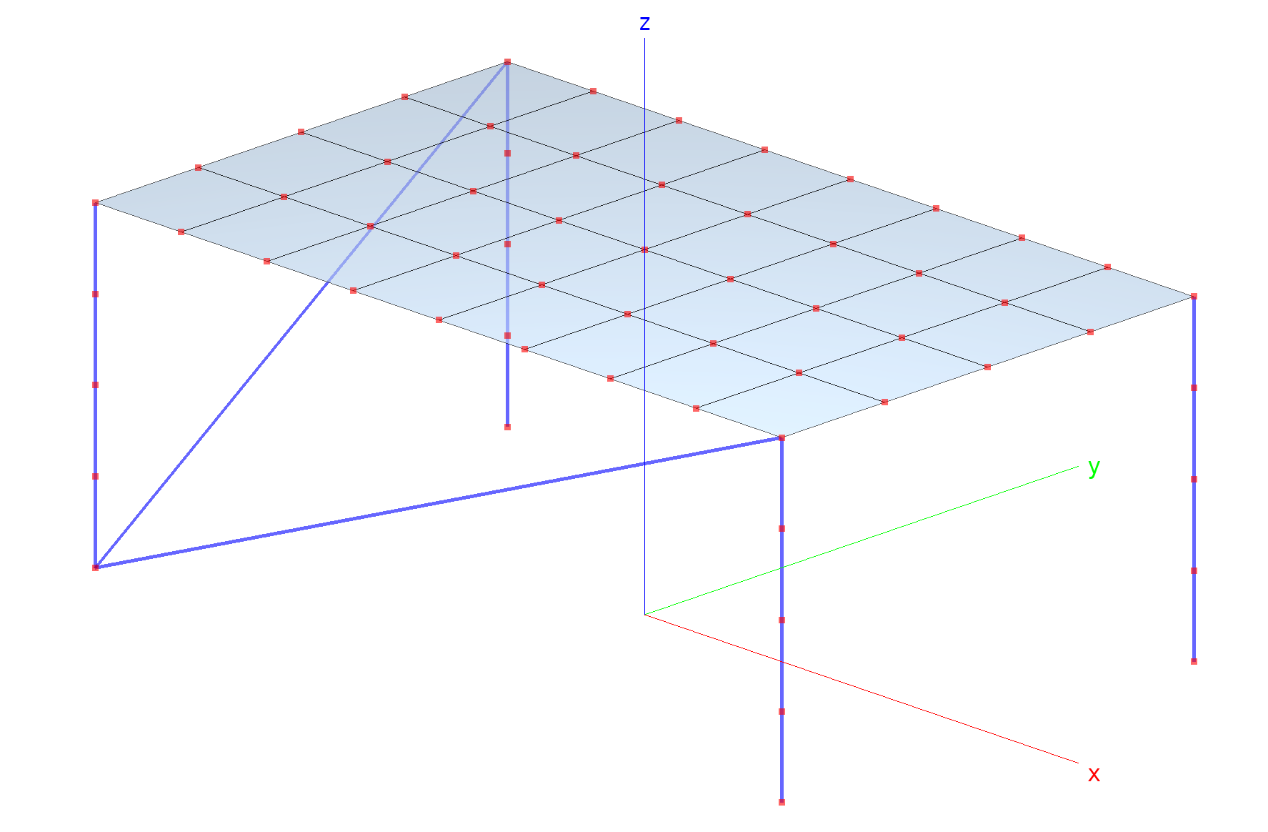
Mixed problem: Mesh generated with the Simples modeler and viewed
with the baspl++ script bv-view-mesh.py).
The plate is loaded with a pressure load of 5000 Pa. The columns are clamped at the base.
The MDL input file mixed.mdl is generated with the Simples
model generation script mixed.py. mixed.py also
launches the solver.:
python3 mixed.py
mixed.pyalso launches the solver, producings the modeldatabase mixed.b2m.
The post-processor (baspl++) scripts bv-view-mesh.py display
the mesh and bv-view-deformed.py the deformed shape:
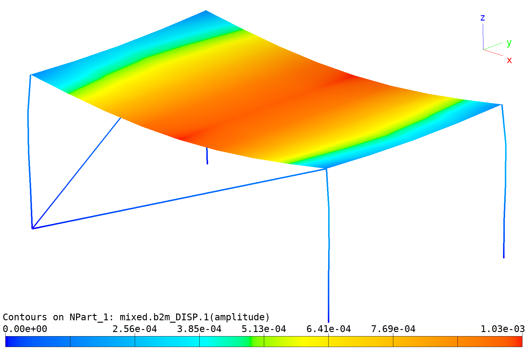
Mixed problem: Deformed shape.
In the current version of B2000++ (4.4) beam stresses cannot be computed with the B2000++ solver. This is illustrated in the figure below displaying the failure index: Beam elements are gray (no failure index found).
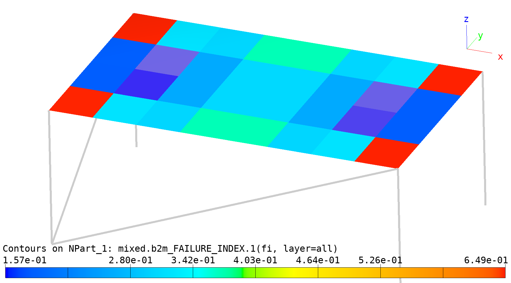
Mixed problem: Failure index.
Beam stresses must be evaluated in a post-processing step with
Simples. The stress extraction script
print_beam_rod_stresses.py illustrates this step: It computes
beam section stresses and prints them for one of the columns of the
model. It also prints the maximum of \(\sigma_{xx}\) (min and
other components are extracted similarly with the
get_max() and
get_min() functions).
"""Simples script to extract and print beam and rod stresses from
"mixed" model."""

import sys
import numpy
import simples as si

def print_beam_stresses(model, elset=None, branch=1, case=1, cycle=0):
    """Computes and prints beam section stresses for all elements of list
    ``elset``.

    """
    field = si.BeamStressField(model, branch=branch, case=case, cycle=cycle)
    if field is None:
        print(f"Beam stress field not found")
        return
    for r in field.get_stresses(elset):
        print(f"Beam stresses, element {r.eid}")
        print(f"   {'ip':>2} {'i':>2} {'sxx':^10} {'st':^10}")
        for ip, stress in enumerate(r.stresses):
            for i, s in enumerate(stress):
                print(f"   {ip:2d} {i:2d} {s[0]:10.4g} {s[1]:10.4g}")

def print_rod_stresses(model, elset=None, branch=1, case=1, cycle=0):
    """Computes and prints rod axial stresses for all elements of list
    ``elset``.

    """
    field = si.SamplingPointField(model, 'STRESS_SECTION_ROD', branch=branch, case=case, cycle=cycle)
    if field is None:
        print(f"Rod stress field not found")
        return
    if elset is not None:
        _eids = tolist(elset)
    else:
        _eids = model.get_branch().get_elem_eids()
    for eid in _eids:
        elstresses = field.get(eid)
        if elstresses is not None:
            print(f"Rod stresses, element {eid}\n   {'ip':>2} {'sxx':^10}")
            for ip, stress in enumerate(elstresses):
                 print(f"   {ip:2d} {stress[0]:10.4g}")

dbname = ('mixed.b2m' if len(sys.argv) < 2 else sys.argv[1])

model = si.Model(dbname)

# Compute beam stresses for the first column "column1". Columns 2-4
# idem.

elset = model.get_elem_set("column1")
print_beam_stresses(model) # prints all element stresses
#-demo :print_beam_stresses(model, elset) # prints all beam element stresses of elset
print_rod_stresses(model) # prints all rod element stresses of elset
Executing the script with Python3:
python3 print_stresses.py

Beam stresses, element 1
   ip  i    sxx         st
    0  0 -1.665e+07          0
    0  1 -1.131e+07          0
    0  2 -1.665e+07          0
    0  3 -1.382e+07          0
Beam stresses, element 2
   ip  i    sxx         st
    0  0 -1.195e+07          0
    0  1 -1.275e+07          0
    0  2 -1.195e+07          0
    0  3 -1.238e+07          0
Beam stresses, element 3
   ip  i    sxx         st
    0  0  -7.24e+06          0
    0  1  -1.42e+07          0
    0  2  -7.24e+06          0
    0  3 -1.093e+07          0
Beam stresses, element 4
   ip  i    sxx         st
    0  0 -2.536e+06          0
    0  1 -1.564e+07          0
    0  2 -2.536e+06          0
    0  3 -9.487e+06          0
Stress max(Sxx) in element smax[0], sxx= 1.051e+06
2.6. Node-Local Transformation
Folder: B2EXAMPLES/static/node_local_transformation
This basic test explains the local orientations of values at nodes, such as boundary condition or DOF values. The test model is a cantilever beam modeled with 4 B2.S.RS beam elements. It is clamped at node 1 and loaded with a force in the global y direction at node 5. Three nodes are defined in a local system by defining transformations
transformations
  # Transformation 3: Rotation around z-axis by -90 deg
  3 cartesian  0. 0. 0.  0. 0. 1.  0. -1 0. # x_local = -y

  # Transformation 5: Rotation around z-axis by 90 deg, x_local = y: Ux_local = Uy_global
  5 cartesian  0. 0. 0.  0. 0. 1.  0. 1. 0.
end
and assigning them to nodes
nodes
  1 0. 0. 0.
  2 2.5 0. 0.
  transformation 3
  3 5. 0. 0.
  transformation 0 # Restore global
  4 7.5 0. 0.
  transformation 5
  5 10. 0. 0.
end
The node-local Cartesian coordinate systems of boundary conditions and DOF values of the mesh nodes are as follows:
Node 1 has (default) global orientation (no transformation).
Node 2 DOF values are defined in the local system of transformation 3. Since no boundary conditions are define at node 3 no transformation will be applied by the solver.
Node 4 has (default) global orientation (no transformation).
Node 5 has the assigned local transformation 5: DOF 1 points to the global direction y, DOF 2 to global direction -x, and DOF 3 to global direction z. Transformations will be applied by the solver.
Beam mesh (black). Nodes marked by black squares. Local orthogonal
coordinate systems (red: x-axis, green: y-axis, blue:
z-axis). baspl++ script bv-node-local-coordinate-systems.py
generates this plot.
nbc and ebc conditions must be formulated and input in the node-local system. Thus, defining an applied force (value=30) in the global y-direction with the nbc command
# Applied force Fy in global y-direction (DOF 2). Local: Fx (DOF 1)
nbc 1
  value 30 dof Fx nodes 5
end
requires to assign the force to DOF 1 due to the local transformation.
Results are by default generated and stored with respect to the (branch) global system. For node 5 the generated applied forces are stored on the database in the (branch) global system:
Node |
Sys |
Fx |
Fy |
Fz |
Mx |
My |
Mz |
|---|---|---|---|---|---|---|---|
5 |
G |
0 |
30 |
0 |
0 |
0 |
0 |
Likewise, the resulting displacements and rotations are stored on the database in the (branch) global system:
Node |
Sys |
Ux |
Uy |
Uz |
Rx |
Ry |
Rz |
|---|---|---|---|---|---|---|---|
5 |
G |
0 |
1.078 |
0 |
0 |
0 |
0.15 |
Print DOF result with b2print_solution in (default) global system:
b2print_solutions beam.b2m

Field "DISP": Displacements and Rotations
case=1, cycle=0, DOFs in global system
Selected set="All nodes"

      EID           Ux           Uy           Uz           Rx           Ry           Rz
        1            0            0            0            0            0            0
        2            0       0.1054            0            0            0      0.06563
        3            0       0.3515            0            0            0       0.1125
        4            0       0.6913            0            0            0       0.1406
        5            0        1.078            0            0            0         0.15
Print DOF result with b2print_solution in local system (nodes 3 and 5):
b2print_solutions --local beam.b2m

Field "DISP": Displacements and Rotations
case=1, cycle=0
Selected set="All nodes"

      EID           Ux           Uy           Uz           Rx           Ry           Rz        Local
        1            0            0            0            0            0            0            g
        2            0       0.1054            0            0            0      0.06563            g
        3      -0.3515            0            0            0            0       0.1125            l
        4            0       0.6913            0            0            0       0.1406            g
        5        1.078            0            0            0            0         0.15            l
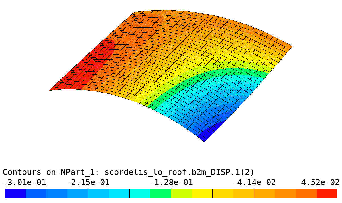
2.7. Scordelis-Lo Roof (Cylindrical Shell)
Folder: file:$B2EXAMPLES/static/scordelis_lo_roof
The Scordelis-Lo roof is a classical test case for linear static analysis named after the authors who first reported it [scordelis]. The test has been proposed as a standard FE test by MacNeal and Harder [macneal1985] and it can be found in the NAFEMS test case description.
The structure consist of a concrete cylindrical shell roof supported by rigid diaphragms on both curved sides (see figure below), and it is loaded by a surface traction of 90psf in the negative y-direction. The total length of the cylinder is 50ft, the radius of the cylinder 25ft, the half opening angle 40°, and the thickness 0.25 ft. The material properties are isotropic, with the elastic modulus of 4.32e8psf and the Poisson number set to 0 or, in some references, to 0.17. Von Mises failure stress is 300000psf.
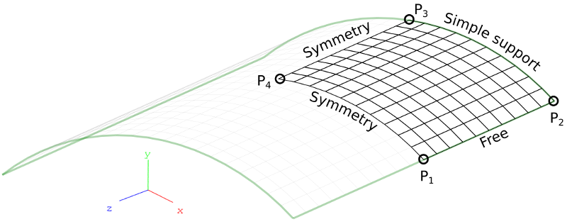
Scordelis-Lo Roof: Mesh.
The diaphragms are defined such that a simply supported boundary condition results: Displacements in x- and y-directions are suppressed, the suppression of displacements in the z-direction being assumed by the symmetry condition along \(P_4\)-\(P_1\).
The test compares the linear static solution, specifically the displacement in the y-direction of point \(P_4\), against known solutions (the reference solution for point \(P_4\) is -0.3024).
The solution of this problem with B2000++ consist of the following steps:
- Create the finite element model with the MDL language describing the
problem in a text file
scordelis_lo_roof.mdl.
Solve the problem by submitting the text file to the B2000++ solver. The solver creates a B2000++ database.
Examine the results by reading the B2000++ database.
A finite element model for B2000++ is created by describing the problem geometry, creating a finite element mesh, adding boundary conditions, and adding solver instructions. The complete model can be formulated with the B2000++ Model Description Language (MDL). Alternatively, parts of the model, such as the mesh and the boundary conditions, can be produced with an external program and brought in the B2000++ input file.
The Scordelis-Lo roof problem can easily be produced with the B2000++ Model Description Language. The necessary steps will now be explained. All steps result in instructions added with an editor to a single B2000++ input file.
Geometry and mesh: The cylinder geometry and the mesh produced by
the geometry can be described with an epatch (element
patch). Element patches allow for generating simple building blocks,
such as plates, cylinders, etc. The Scordelis-Lo cylindrical roof is
described by an epatch of type cylinder, which implies the
creation of a surface and a surface mesh:
epatch 1
    geometry cylinder
    type (ELTYPE)     # Element typ
    ne1 (NE) ne2 (NE) # N. of elements along sides
    thickness 0.25    # Thickness of shell
    mid 1             # Material identifier
    phi1 50.0         # Opening angle of half cylinder
    phi2 90.0         # Closing angle of half cylinder
    radius 25.0       # Radius of cylinder
    length 25         # Half length of cylinder
    # local edges means that all DOF's of the nodes along the edges are
    # expressed in local, i.e. cylindrical, coordinates.
    if (local == 1) {local edges}
end
Note that the epatch must contain the element type (eltype
keyword), the number of elements to be generated along each side of
the patch (ne1 and ne2 keywords), and material reference
(mid keyword). The definition of the epatch is further
illustrated in the figure below, with the position of the vertices P1
to P4 and the edges E1 to E4. Default parameters for the epatch are:
ELTYPE: Q4.S.MITC
NE: 8 (generates 8 by 8 mesh)
GRADIENT: -1 (Gradients at last step)
In this particular configuration the local and global orientations are
the same, i.e. no need to define cylindrical coordinates, unless the
resulting displacements, rotations, forces, and moments should be
expressed in cylindrical coordinates (see instruction if (local
== 1) {local edges} above).
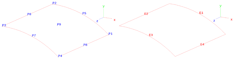
Scordelis-Lo Roof: epatch vertex points and edge
definitions. See also the generated mesh.
Material: The material is the same as the one in the original
problem description. The definition is straightforward with the
material'' command, which identifies the material with id ``1
material 1
    type isotropic
    e 4.32e8       # Young's modulus
    nu 0.          # Poisson number
    density 90
    failure von_mises
      r 300000
    end
end
Boundary conditions: Since all boundary conditions apply either to
edges of the epatch or to the epatch surface they can be
generated for all nodes of an edge by referring to the epatch edges
which in their turn are automatically generated. Essential boundary
conditions (here: displacement constraints) are defined with the ebc
command:
ebc 1
    value 0 # Values to be assigned to DOF's
    # Diaphragm = Supported edge (global=local orientation) along
    # edge e1 from P1 to P2
    dof [UX UY] epatch 1 e1
    # Symmetry condition along edge e2 from P2 to P3
    dof [UX RY RZ] epatch 1 e2
    # Symmetry condition along edge e3 from P3 to P4
    dof [UZ RX RY] epatch 1 e3
end
The figure below shows the essential boundary conditions as defined
above: At each node of the edges a pattern XXXXXXX is plotted,
where the position of X in the pattern designates the degree of
freedom (DOF) to be affected and X taking the values F (free,
i.e. unconstrained), L (locked, i.e. constrained to 0), or V
(constrained to a value).
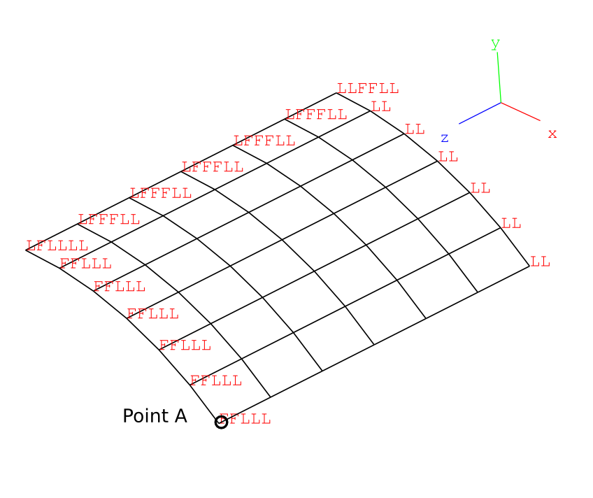
Scordelis-Lo Roof: Essential boundary conditions generated by ebc
1.
The surface pressure loads are applied with the natural boundary
condition command nbc. Note that the reference frame for the surface
tractions is the branch reference frame and thus has to be specified
explicitly with the system option, because the default reference frame
is the local reference frame relative to the element surface.
nbc 1 type surface_tractions
system branch # Branch referential (default is local!)
surface_tractions 0 -90 0
epatch 1 f7 # Apply to mid-surface of shell!
end
What remains now to be specified are (1) definition of the case, comprising the type of analysis (2) the boundary condition sets to be applied to the case (3) the analysis directives, i.e. the cases to be solved for:
case 1
analysis linear
nbc 1
ebc
1
end
adir
case 1
end
The analysis is run with the shell command:
b2000++ scordelis_lo_roof.mdl
which generates the B2000++ database
scordelis_lo_roof.b2m. Specifying the log option to the
b2000++ command prints a short summary of the steps which the solver
performs:
$ b2000++ -l info scordelis_lo_roof.mdl
INFO:all:13:57:24.656: Start
INFO:solver.static_linear:13:57:24.658: Start static linear solver
INFO:domain:13:57:24.658: Total number of DOfs: 422.
INFO:solver.static_linear:13:57:24.659: Element matrix assembly
INFO:solver.static_linear:13:57:24.660: Resolve the linear problem
INFO:solver.static_linear:13:57:24.664: Compute gradients and reaction forces
INFO:solver.static_linear:13:57:24.664: End of static linear solver
INFO:all:13:57:24.664: End of execution
Results
The summary of the analysis results for the 8 by 8 element mesh is displayed in the table below for element type Q4.S.MITC.E4:
What |
Reported |
B2000++ |
Error (%) |
|---|---|---|---|
Displacement DY at point P3 [ft] |
-0.3024 |
-0.304196 |
0.6 |
Results can be examined with several B2000++ tools, such as the
baspl++ post-processor,
the Simples scripting tools, the
*b2print_ text output tools, or the B2000++ data browser. We start with the baspl++ viewer to get an
image of deformed shape of the structure. The figure below is obtained
by launching baspl++ from the shell with the viewer script
view.py:
baspl++ -t plot_displacements.py
and shows the deformed structure (colored) and the initial undeformed
one (black dashed grid). Please read the file view.py.
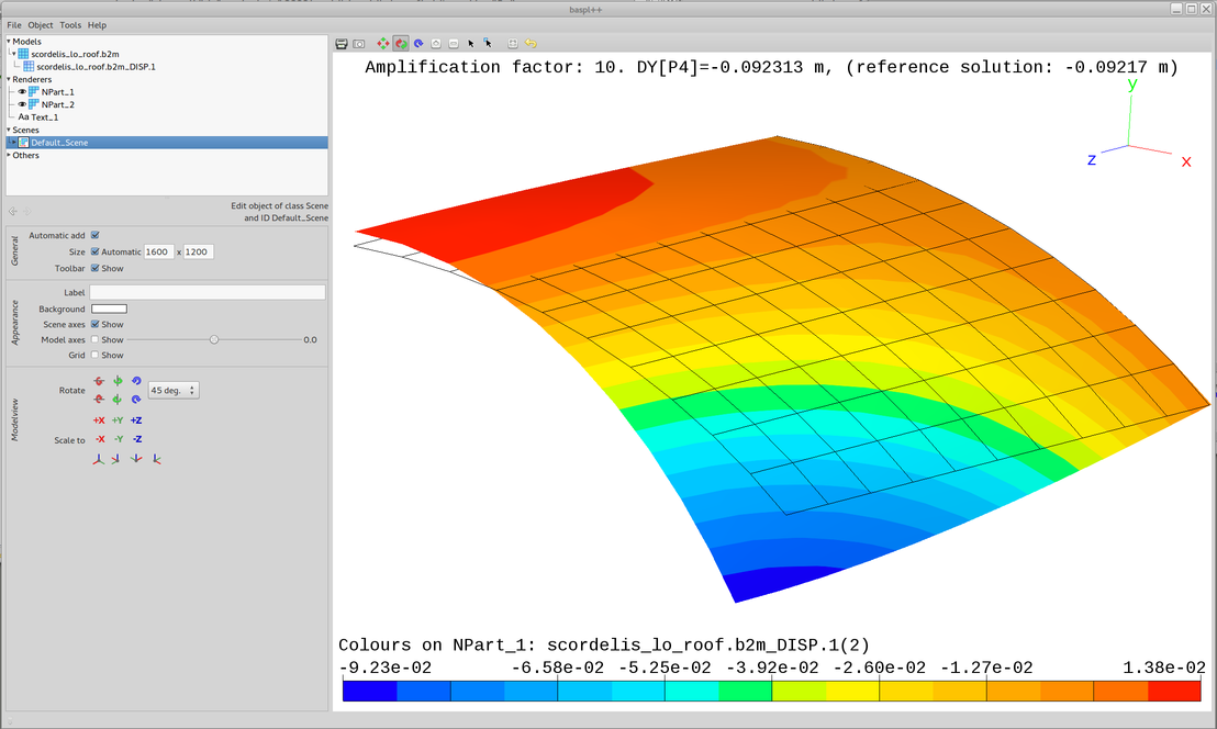
Scordelis-Lo Roof: Displacement field.
baspl++ -t plot_stresses.py
plots the per element maximum von Mises comparison stress:
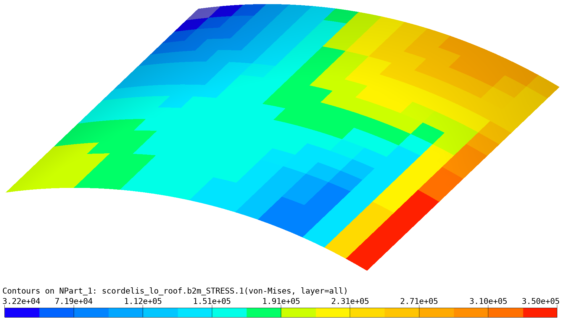
Scordelis-Lo Roof: von Mises stresses (max of element).
baspl++ -t plot_stresses_sampling.py
plots the von Mises comparison stress at each integration (sampling) point in the form of spheres, where color and sphere size are proportional to the intensity:
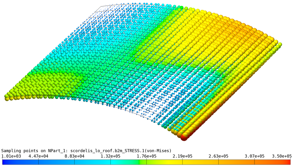
Scordelis-Lo Roof: von Mises stresses (all sampling points).
Values can be extracted with Simples scripts. The script
print_displacement.py extracts the displacement at point P3 and
prints it:
python print_displacement.py
producing the output
Displacement at point P3 (node 273): DY=-0.301733
Reference solution DYREF=-0.3024
Error=-0.22%
and the script print_stresses.py extracts and prints stress
values at selected elements prints it:
python3 print_vmises.py

Max failure index fmax=1.124541, element=241
Data can be viewed with the B2000++ data browser. Example: View the failure index:
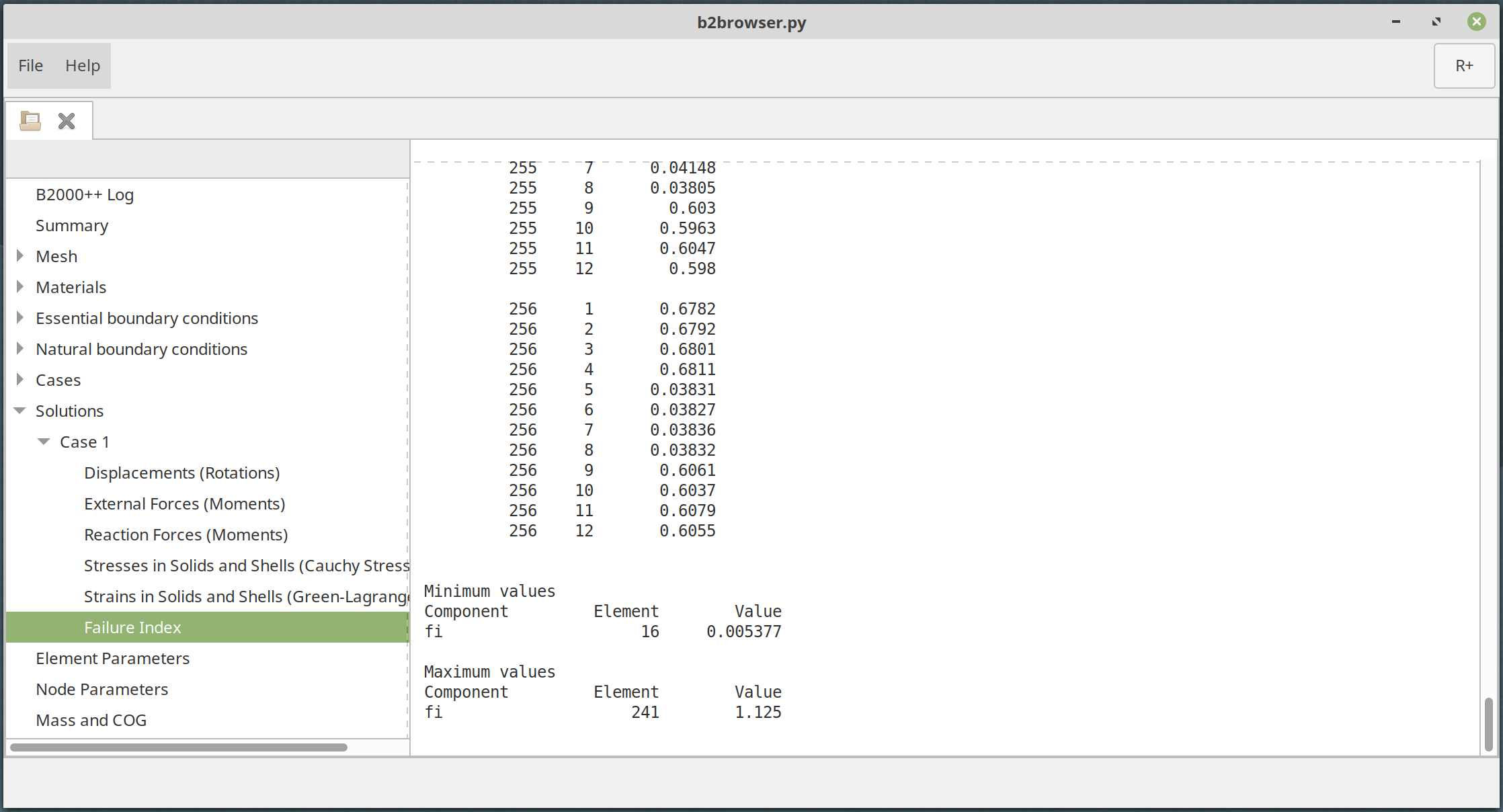
Scordelis-Lo roof: View failure index values with the B2000++ browser.
A convergence study increasing the number of cells (mesh density) with
Simples scripting is very easily performed (script
convergence.py). The graph produced by the script is displayed
below:

Scordelis-Lo roof: Convergence graph for selected element types.
The baspl++ viewer allows for off-screen (batch mode) rendering. Batch
mode is particularly useful if images are to be generated on a plaform
without graphic rendering. Batch mode must be launched with a script
(see example script plot_displacements_batch.sh).
File “output.png” produced in batch mode by script “plot_displacements_batch.sh”.
2.8. New Beam Cross Section Solver (from Version 4.6.6)
Folder: $B2EXAMPLES/static/sectionproperties
This example demonstrates how the new beam cross section solver based
on the sectionproperties package works.
The test is a clamped beam B2000++ model channel.mdl (not listed
here). The beam is loaded with end loads:
Case |
Load |
|---|---|
1 |
End load Fx |
2 |
End load Fy |
3 |
End load Fz |
4 |
End moment Mxx |
The model makes use of B2.S.RS beam elements with one gradient
integration point (constant forces and moment over the beam element).
The beam cross section is defined with the new B2000++ beam property
type sectionproperty, see channel.mdl. The section definition
section "channel_section(d=0.084836, b=0.03556, t_f=0.004318, t_w=0.004318, r=0.0, n_r=0)"
is the one of sectionproperties. Specification of the beam property 1:
property 1
  type sectionproperty
  # Nastran channel_section (sectionproperty): r=0.0 and n_r=0 mean no "root radius"
  # meshsize=0.0 means default mesh size selcted by sectionproperties.
  section "channel_section(d=0.084836, b=0.03556, t_f=0.004318, t_w=0.004318, r=0.0, n_r=0)"
  meshsize=0.0
  mid 1
end
After execution of the B2000++ input processor
b2ip++ channel.mdl
you can inspect the beam cross section meshes generated by
sectionproperties. The Simples app b2plot_section_properties will
plot section geometries and section solver meshes. Example plot of
property 1:
b2plot_section_properties --save channel.b2m 1

***INFO: Created file "section-geometry,pid=1.svg"
***INFO: Created file "section-mesh-and-centroid,pid=1.svg"
The 0 in the above command generates the 2 section plot files section-1-g.svg (cross section
solver FE geomety) and section-1-c.svg (computed centroid and
shear center) of all defined sections (here: section=pid=1):

sectionproperties channel section geometry of property PID=1. |

sectionproperties channel section geometry of property PID=1. |
Thereafter you can solve for the given load cases with
b2000++ channel.b2m
B2000++ solves for displacements, rotations, and gradients (section forces and moments, NOT* beam stresses!). The diagrams below display displacements ux (DOF 1), uy (DOF 2), uz (DOF 3), and rotations rx (DOF 4), ry (DOF 5), rz (DOF 6).

Displacements ux, uy, uz and rotations rx, ry, rz over beam x-axis.
Beam section stresses can now be computed with the
b2print_beamstresses app. By default prints element min and max
stresses at all integration points IP for all elements. Element 0
means overall values Example: Compute and format to a text file
stresses for case 1 and component sxx, processing all
elements.
b2print_stresses_beams --case=3 channel.

Element stresses
EID  IP       SXX-MIN      SXX-MAX       SYX-MIN      SYX-MAX        SZX-MIN      SZX-MAX      SYZ-MIN      SYZ-MAX          SVM   FINDEX
  1   0 -6.448935e+06 6.448935e+06 -1.283106e+06 1.283106e+06 -811864.579023 1.343997e+06 40171.866056 1.343997e+06 6.691222e+06 0.048487
  2   0 -6.284566e+06 6.284566e+06 -1.283106e+06 1.283106e+06 -811864.579023 1.343997e+06 40171.866056 1.343997e+06 6.532952e+06 0.047340
  3   0 -5.962281e+06 5.962281e+06 -1.283106e+06 1.283106e+06 -811864.579023 1.343997e+06 40171.866056 1.343997e+06 6.223542e+06 0.045098
  4   0 -5.639995e+06 5.639995e+06 -1.283106e+06 1.283106e+06 -811864.579023 1.343997e+06 40171.866056 1.343997e+06 5.915508e+06 0.042866
  5   0 -5.317710e+06 5.317710e+06 -1.283106e+06 1.283106e+06 -811864.579023 1.343997e+06 40171.866056 1.343997e+06 5.609075e+06 0.040645
  6   0 -4.995424e+06 4.995424e+06 -1.283106e+06 1.283106e+06 -811864.579023 1.343997e+06 40171.866056 1.343997e+06 5.304522e+06 0.038439
  7   0 -4.673139e+06 4.673139e+06 -1.283106e+06 1.283106e+06 -811864.579024 1.343997e+06 40171.866057 1.343997e+06 5.002191e+06 0.036248
  8   0 -4.350853e+06 4.350853e+06 -1.283106e+06 1.283106e+06 -811864.579024 1.343997e+06 40171.866057 1.343997e+06 4.702512e+06 0.034076
  9   0 -4.028568e+06 4.028568e+06 -1.283106e+06 1.283106e+06 -811864.579024 1.343997e+06 40171.866057 1.343997e+06 4.406024e+06 0.031928
 10   0 -3.706283e+06 3.706283e+06 -1.283106e+06 1.283106e+06 -811864.579024 1.343997e+06 40171.866057 1.343997e+06 4.113419e+06 0.029807
 11   0 -3.383997e+06 3.383997e+06 -1.283106e+06 1.283106e+06 -811864.579024 1.343997e+06 40171.866057 1.343997e+06 3.825588e+06 0.027722
 12   0 -3.061712e+06 3.061712e+06 -1.283106e+06 1.283106e+06 -811864.579024 1.343997e+06 40171.866057 1.343997e+06 3.543694e+06 0.025679
 13   0 -2.739426e+06 2.739426e+06 -1.283106e+06 1.283106e+06 -811864.579023 1.343997e+06 40171.866056 1.343997e+06 3.317078e+06 0.024037
 14   0 -2.417141e+06 2.417141e+06 -1.283106e+06 1.283106e+06 -811864.579023 1.343997e+06 40171.866056 1.343997e+06 3.108416e+06 0.022525
 15   0 -2.094855e+06 2.094855e+06 -1.283106e+06 1.283106e+06 -811864.579024 1.343997e+06 40171.866056 1.343997e+06 2.913603e+06 0.021113
 16   0 -1.772570e+06 1.772570e+06 -1.283106e+06 1.283106e+06 -811864.579024 1.343997e+06 40171.866056 1.343997e+06 2.735601e+06 0.019823
 17   0 -1.450284e+06 1.450284e+06 -1.283106e+06 1.283106e+06 -811864.579022 1.343997e+06 40171.866056 1.343997e+06 2.577894e+06 0.018680
 18   0 -1.127999e+06 1.127999e+06 -1.283106e+06 1.283106e+06 -811864.579022 1.343997e+06 40171.866056 1.343997e+06 2.461823e+06 0.017839
 19   0 -8.057136e+05 8.057136e+05 -1.283106e+06 1.283106e+06 -811864.579021 1.343997e+06 40171.866056 1.343997e+06 2.382357e+06 0.017263
 20   0 -4.834282e+05 4.834282e+05 -1.283106e+06 1.283106e+06 -811864.579020 1.343997e+06 40171.866056 1.343997e+06 2.327874e+06 0.016869
 21   0 -1.611427e+05 1.611427e+05 -1.283106e+06 1.283106e+06 -811864.579019 1.343997e+06 40171.866056 1.343997e+06 2.327871e+06 0.016869

 Overall Element stresses minmax
       SXX-MIN      SXX-MAX       SYX-MIN      SYX-MAX        SZX-MIN      SZX-MAX      SYZ-MIN      SYZ-MAX          SVM   FINDEX
 -6.448935e+06 6.448935e+06 -1.283106e+06 1.283106e+06 -811864.579024 1.343997e+06 40171.866056 1.343997e+06 6.691222e+06 0.048487
Finally, beam stresses can be visualized with the
sectionproperties stress plot utility, through the Simples app
b2plot_section_stresses. Example: Plot \(\sigma_{xx}\) contours
over the section for element 1 and load case 3:
b2plot_stresses -e=1 --case=3 --save channel.b2m

***INFO: Created file "beam_section_stresses_eid=1,case=3,cycle=None,comp=sxx.svg"
***INFO: Created file "beam_section_stresses_eid=1,case=3,cycle=None,comp=svm.svg"

\(\sigma_{xx}\) stress contours for load case 3, element 1.

\(\sigma_{xx}\) stress contours for load case 3, element 1. |

\(\sigma_{vm}\) stress contours for load case 3, element 1. |
2.9. Linear Analysis with Subcases
Folder: $B2EXAMPLES/static/subcases
Th example illustrates the concept of subcases (see case definition). During linear analysis, subcases can be applied to a common set of essential boundary conditions, thus reducing solution time, because the constraints are applied once and the global matrix is factored once. Each subcase is a new right-hand side and needs back-substitution only.
The model is the same as the Buckling of Composite Plate example: A simply-supported thin quadratic laminated plate of 500 mm by 500 mm is loaded with 2 load cases and same essential boundary conditions.
The first load case (case 100) constrains the plate to simply supported condition (essential boundary condition 1). Under this condition, 2 natural boundary conditions (nbc) force sets are applied as subcases:
case 100
    analysis linear
    gradients 1
    ebc 1
    subcase 1 # Subcase 1: Pressure load (nbc 1)
        nbc 1
    end
    subcase 2 # Point load applied at the plate's mid-point (nbc 2)
        nbc 2
    end
end
The second load case (case 200) is the same as case 100 and serves as test for subcase reference.
case 100
    analysis linear
    gradients 1
    ebc 1
    subcase 1 # Pressure load (nbc 1)
        nbc 1
    end
    subcase 2 # Point load at mid-node
        nbc 2
    end
end

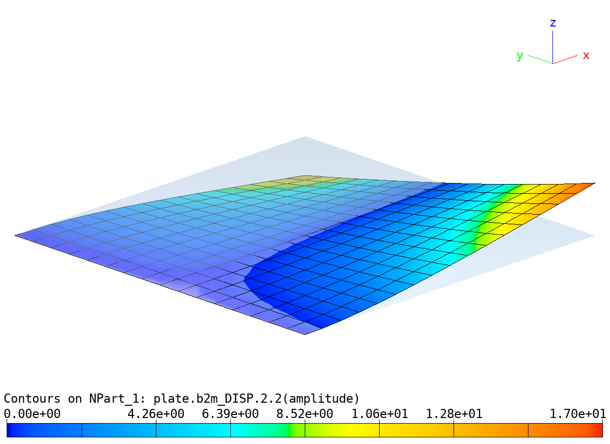
Geometry and essential boundary conditions of plate.
Note that B2000++ always solves for all subcases of a case, i.e specifying
adir
    cases [100 200]
end
will solve for subcase 1 and subcase 2 of cases 100 and 200.
The input file plate.mdl contains all definitions for solving the
2 cases with 2 subcases each. The essential and natural boundary
condition definitions are not listed here (see MDL input file
plate.mdl).
The deformed shapes of the subcases are displayed in the figures
below. Note that the selection of the subcase in baspl++ and
Simples is obtained with the subcase= or mode= parameter.
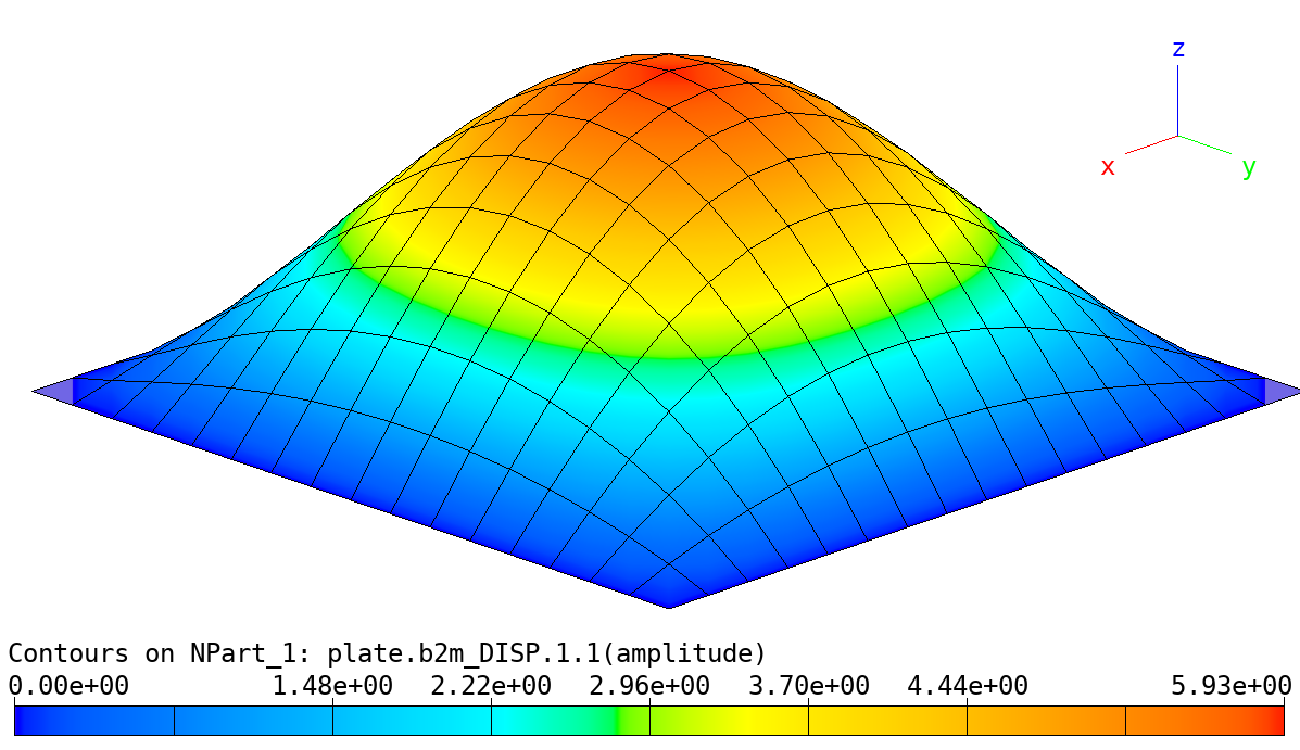
Linear Analysis of Plate with subcases: Amplified deformed shape, case 1, subcase 1.
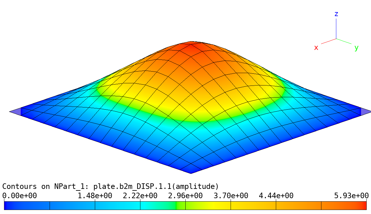
Linear Analysis of Plate with subcases: Amplified deformed shape, case 1, subcase 2.
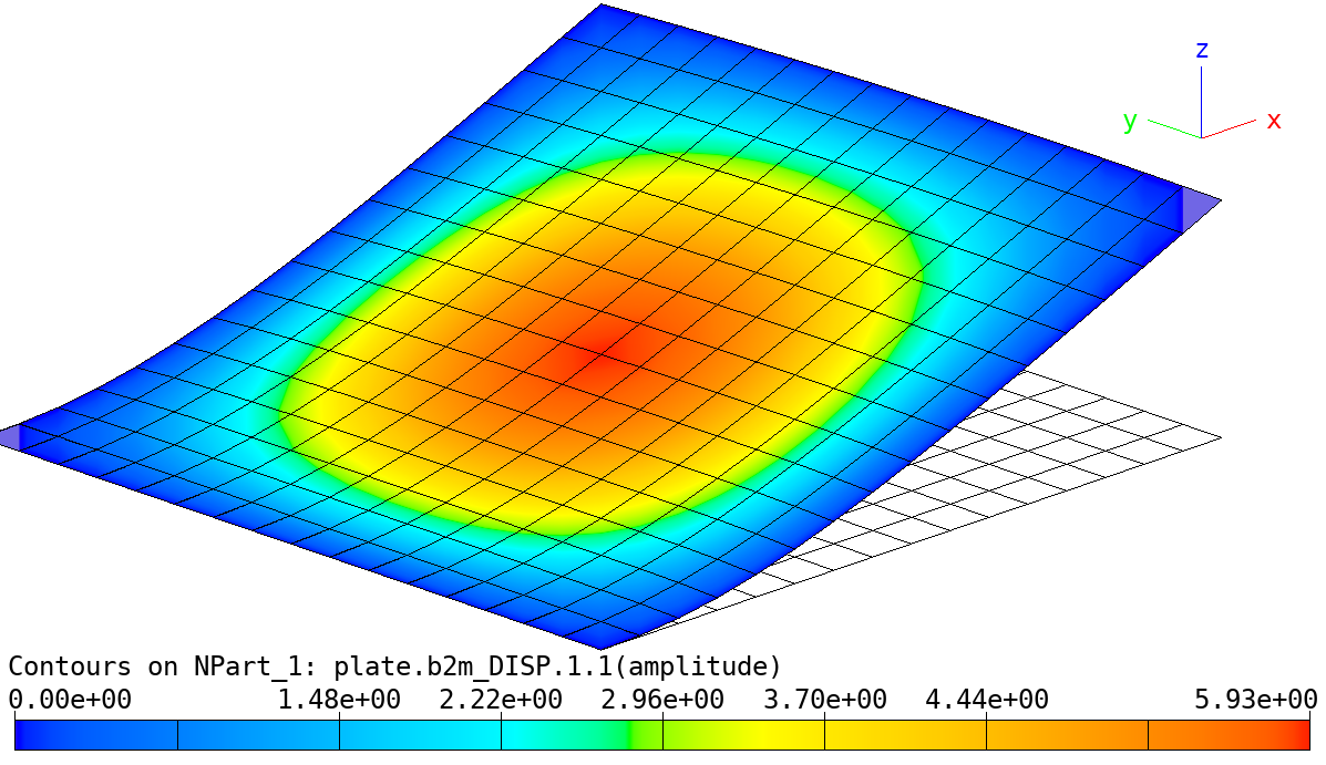
Linear Analysis of Plate with subcases: Amplified deformed shape, case 2, subcase 1.
Linear Analysis of Plate with subcases: Amplified deformed shape, case 2, subcase 2.
Execute the test with
b2000++ plate.mdl
Solutions can the be examines with b2print_solutions``. Example: Print the displacements and rotations of mid-node 128 for case 200 and subcase 2:
b2print_solutions --case=200 --subcase=2 --item=128  plate.b2m/

DOF Field "DISP", mesh=1, case=200, cycle=0, subcase=2, selection="Selected nodes"
EID           Ux           Uy           Uz           Rx           Ry           Rz
128     2.24e-21    -1.52e-20        2.128     0.001757     -0.01189            0
Plot the deformed shape with baspl++ script bv-deform.py.
Finally, the test runner executes the test and heck the force and
displacement results (see __init__.py. Execute from the test
directory with the shell:
b3tesrunner .
2.10. Cylinder modeling using axisymmetric elements
Folder: $B2EXAMPLES/static/axisym
This example demonstrates working with axisymmetric elements to model a cylinder subjected to a specific inner pressure. The cylinder is fixed in axial direction at \(y=0\) (local z-Coordinate) and \(y=L\). The model consists of 7 quadrilateral (Q4) elements in axial direction with only one element in radial direction.
Dimensions and material parameters of the cylinder model:
L = 0.8    # Length of cylinder [m]
R = 0.2    # Radius of cylinder [m]
t = 0.005   # Thickness of cylinder [m]
p = 1.e6   # Pressure [N/m]
E = 72.4e9 # Young's modulus [N/m2]

Cylinder model using axisymmetric elements
Run the one model with:
sh ./run.sh rectangle

   "DISP": Displacements and Rotations
   mesh=1, case=1, cycle=0
   selection="All nodes"

      EID           Ux           Uy
        1    1.029e-05    3.794e-33
        2    1.018e-05    3.746e-33
        3    1.018e-05   -3.746e-33
        4    1.029e-05   -3.794e-33
        5    1.018e-05   -6.737e-20
        6    1.018e-05    -1.06e-19
        7    1.018e-05   -2.535e-19
        8    1.018e-05   -3.729e-19
        9    1.018e-05   -2.644e-19
       10    1.029e-05   -2.418e-19
       11    1.029e-05    -5.37e-19
       12    1.029e-05   -1.896e-19
       13    1.029e-05   -4.854e-20
       14    1.029e-05   -1.301e-19

   "STRESS": Cauchy/linear stress, global reference frame
   mesh=1, case=1, cycle=0
   selection="All elements"

    IDENT           IP          Sxx          Syy          Szz          Sxy          Syz          Sxz
        9            1   -2.722e+04    1.207e+06    4.051e+06   -4.976e-07            0            0
        9            2   -7.051e+04    1.164e+06    3.949e+06   -4.942e-07            0            0
        9            3   -2.722e+04    1.207e+06    4.051e+06   -9.405e-08            0            0
        9            4   -7.051e+04    1.164e+06    3.949e+06   -9.084e-08            0            0
       10            1   -2.722e+04    1.207e+06    4.051e+06    3.396e-07            0            0
       10            2   -7.051e+04    1.164e+06    3.949e+06    3.416e-07            0            0
       10            3   -2.722e+04    1.207e+06    4.051e+06   -4.336e-07            0            0
       10            4   -7.051e+04    1.164e+06    3.949e+06   -4.314e-07            0            0
       11            1   -2.722e+04    1.207e+06    4.051e+06    2.792e-07            0            0
       11            2   -7.051e+04    1.164e+06    3.949e+06     2.75e-07            0            0
       11            3   -2.722e+04    1.207e+06    4.051e+06    2.389e-07            0            0
       11            4   -7.051e+04    1.164e+06    3.949e+06    2.334e-07            0            0
       12            1   -2.722e+04    1.207e+06    4.051e+06   -5.549e-07            0            0
       12            2   -7.051e+04    1.164e+06    3.949e+06   -5.513e-07            0            0
       12            3   -2.722e+04    1.207e+06    4.051e+06    9.126e-07            0            0
       12            4   -7.051e+04    1.164e+06    3.949e+06    9.148e-07            0            0
       13            1   -2.722e+04    1.207e+06    4.051e+06   -3.577e-07            0            0
       13            2   -7.051e+04    1.164e+06    3.949e+06   -3.484e-07            0            0
       13            3   -2.722e+04    1.207e+06    4.051e+06   -1.559e-06            0            0
       13            4   -7.051e+04    1.164e+06    3.949e+06    -1.55e-06            0            0
       14            1   -2.722e+04    1.207e+06    4.051e+06    1.275e-06            0            0
       14            2   -7.051e+04    1.164e+06    3.949e+06    1.266e-06            0            0
       14            3   -2.722e+04    1.207e+06    4.051e+06    1.421e-06            0            0
       14            4   -7.051e+04    1.164e+06    3.949e+06    1.412e-06            0            0