The Model Description Language (MDL) is a data driven language for
describing the geometrical, the physical, and the mathematical
properties of a problem, and the numeric parameters for the
solver(s). To enable parametric models, MDL has features such as
variable assignment, substitution, and some flow control statements.
MDL features variable assignment, substitution, and flow
control. These features enable the writing of parametric input
files. This functionality proves useful in a wide range of contexts,
but it cannot replace real programming languages (such as Python).
MDL language elements are placed in text files. These files may be
created with text editors or by means of scripts.
MDL is interpreted as a stream of items which are separated by space
characters and newline characters. It does not matter how many space or
newline characters are present. Example:
Onetwothree4
is equivalent to
Onetwothree4
Items pertaining to the parametric input either begin with a reserved
word or are enclosed in parentheses. Such items are processed and may
expand to new data items. This is illustrated by means of the
following example:
(a=4)Onetothree(a)
The item “(a=4)” assigns the integer value 4 to the variable “a”, and
the item “(a)” expands the current contents of variable “a”. Thus, the
expanded MDL is
Onetothree4
Comments, i.e. explanatory text, begin with the # character and
stretch until the end of the line.
Integer (or int) numbers contain the characters 0-9, possibly prefixed
by the unary operators + or -. Examples:
100-1+1234
Floating-point (or float) numbers have either a decimal point (.),
an exponent (letter e or E, possibly followed by + or -, and followed by
1-3 digits), or both. They may be prefixed by the unary operators + or
-. Examples:
Unquoted character strings begin with an alphabetic character,
followed by an arbitrary number of alphanumeric characters and/or the
dot (.) and underscore (_) characters. Such unquoted character strings
are used for both attribute names and attribute values. Examples:
Lists are sequences of primitive data, usually integer or
floating-point numbers, character strings, or text strings. Lists are
enclosed by square brackets. Example:
[1234]
For longer lists, ranges can be specified inside the list. Example:
[110/20454650]
generates a list of integers in the form of
[11011121314151617181920454650]
A step size can optionally be specified. The following
Portions of MDL can be placed in separate files which can be inserted by
means of the include statement:
includeFILENAME
FILENAME must be a valid file name without any escape
sequences. If it contains spaces, dot characters (.), slash characters
(/), or other special characters, it must be enclosed by single or
double quotes. File names are relative w.r.t. the directory of the MDL
file containing the include statement. Examples:
Variables are assigned by means of the assignment operator = and the
expression must be enclosed by parentheses. Example:
(i=3)
will assign the integer value 3 to the variable i.
Variable names begin with an alphabetical character (a-z, A-Z),
followed by zero or more alphanumeric and/or underscore (_)
characters.
The value that will be assigned to the variable is evaluated from the
expression that follows the assignment operator. From the expression’s
type, the type of the variable is inferred.
The operator ?= assigns only if the variable has not already been
assigned. In conjunction with the -define command-line option, it
can be used to specify default values that can be overridden on the
command line. Example:
Any expression, variable, or constant of one of the aforementioned
data types, when enclosed by parentheses, constitutes a substitution
statement. Example:
The “not” operator has a higher precedence than the “and” and “or”
operators.
The following relational operators yield bool values:
==,!=,<,<=,>,>=
The operands may be of any type. Operands of type bool and int
are converted to type float. Values of type str are always “greater”
than bool and numerical values. Relational operators have higher
precedence than logical operators.
The following arithmetic operators (for expressions of type int and
float) are available. They are listed with increasing precedence (all
of them with higher precedence than relational operators), with the
addition and subtraction operators having the lowest precedence, and
the power operator the highest.
All these operators can be applied to operands of type int and type
float. For binary operators, when both operands are of type int, the
result is also of type int. When both operands are of type float, the
result is also of type float. When one operand is of type int and the
other of type float, the int operand is first converted to a float, and
the result is of type float.
For str expressions, the binary operator + means concatenation:
("A "+"string "+"with "+"several "+"words.")
Sub-expressions may be enclosed in parentheses to override the operator
precedence rules. Example:
The break statement exits the directly enclosing loop. The
continue statement stops the processing of the current iteration of
the loop and continues with the next iteration of the loop. Example:
MDL commands are text blocks describing specific data, such as node
coordinates, material properties, etc. Each block starts with a
keyword and is terminated by end.
Upper case text in the input descriptions of blocks and all other
specifications of this chapter signifies replaceable or variable.
acceleration_init defines initial second time derivatives of DOF fields
(accelerations). The dynamic (transient) or non-stationary solver will
include initial DOF fields at time t = 0. If no initial conditions are
specified the solver will assume all initial conditions to be 0.
An acceleration_init set is identified by IDENT (non-negative int).
IDENT is the number which is referenced by the acceleration_init
options of case. Sets with an identifier of 0 will be active for all
analysis cases. For a detailed description of the parameters see rubric
MDL Specification of the command dof_init.
Examples
Create a uniform acceleration_init (acceleration field) in the global
z-direction. Note that all other DOFs are implicitly set to 0.
acceleration_init 123
   value 5 dof UZ allnodes
end
The field must be activated with the acceleration_init parameters of
case:
adir specifies the analysis cases to be processed and directives
that apply to all analysis cases. adir may only be defined once in
a MDL file.
MDL Specification
adir
  directives...
end
Directives (required)
caseIDENT|cases[IDENT1IDENT2...]
Specifies the analysis case(s) to be processed (required). The
identifier IDENT refers to a specific analysis case, see the case command.
Directives (optional)
add_ssc_elements
Automatically add shell-to-solid coupling (SSC) elements on
interfaces between shell and solid elements. Note that the shell
intersection detection algorithm is inhibited if the -iponly
option is specified in calling the b2000++ input processor.
drillsV
The drill stiffness factor V is used by the MITC shell elements to
stabilize the 6th degree-of-freedom (RZ). The default
value is 1e-8.
shell_intersection_angleV
MITC shell elements only: The node type with 5 or 6
degrees-of-freedom is determined in function of topological and
geometric properties of the Finite Element mesh, as well the
essential boundary conditions. The shell intersection angle V
specifies the minimum angle in degrees (default is 30.0) at which
elements meet. Thus, nodes of elements joining at an angle greater
than v will have 6 degrees-of-freedom.
Note that the shell intersection detection algorithm is inhibited
if the -iponly option is specified in calling the b2000++ input
processor.
symmetry_planePXPYPZNXNYNZ
Specifies a symmetry plane by specifying a point p=(PY,PY,PZ) of
the plane and the normal of the symmetry plane n=(NY,NY,NZ). Up
to 6 symmetry planes can be defined. Note that defining symmetry
planes does not entail that the symmetry planes will be used by
b2000++. Specific solvers, such as the heat analysis radiation
solver, will check for symmetry planes.
atemperatures specifies ambient temperature values at nodes for
defining convective conditions in heat analysis in conjunction with
the heat convection ‘overlay’ elements` defining the set number (a
positive integer). To specify temperatures at nodes inducing thermal
strains in stress analysis, please refer to the command. An
atemperatures set is identified by IDENT, a non-negative integer
which must be unique for the atemperatures conditions of the
current model. IDENT is the number which is referenced by the
atemperatures parameter of the case command. Sets with an
IDENT of 0 will be active for all analysis cases.
MDL Specification
atemperatures ID
  parameters
  node specifications...
end
Parameters
valueV
Specifies the current ambient temperature value V assigned to
subsequently specified nodes.
Node specifications
allnodes
Assign the ambient temperature values to all defined nodes of the
current branch.
branchBR
For models that consist of several branches (deprecated).
Specifies the external branch number br.
To be used in conjunction with the allnodes and nodes directives.
epatchIDPX|EX|FX|B
Selects nodes from an epatch. Individual patch vertex nodes
are specified with the strings P1 to P8. Patch edge nodes
are specified with the strings E1 to E12. Patch face nodes
are specified with the strings F1 to F6. Patch body nodes
of the whole patch body are specified with the string B.
nodeN|nodes[N1N2...]
Specifies a node or a list of nodes (of the current branch) to
which the ambient temperature value will be assigned.
atemperatures generates the dataset(s) ATEMP.br.0.0.<IDENT>.
DEPRECATED in 4.6.5!
Multiple branches will not be supported in future versions of b2000++.
The branch directive remains available, but future versions of b2000++
will only support a single branch (with number 1).
The branch command sets the current branch mesh. All mesh
specifications will pertain to the branch until a new branch
command is issued. If not specified, the default branch is 1: All
MDL specifications thereafter will refer to branch 1.
MDL Specification
branch IDENT
  mesh specification...
end
Additional
A “branch” (or mesh) is a finite element mesh consisting of nodes and
elements and identified uniquely by the mode and element IDENT
(positive integers). Each branch is identified by its unique positive
integer number. The default branch is 1: All model specifications will
refer to branch 1 if not stated otherwise. Note that in newer versions than
4.6.5 there is only a single branch supported in b2000++ anymore.
Most finite element models (including those that were converted from
other finite element codes) consist of a single branch or mesh, and in
this case it is not necessary to specify the mdl.branch command.
Defining multiple branches is deprecated in b2000++ versions newer than
4.6.5.
In the presence of multi-branch (multi-mesh) models, the nodes (and
degrees-of-freedom) between branches (meshes) must be connected with
the mdl.join or the mdl.link commands.
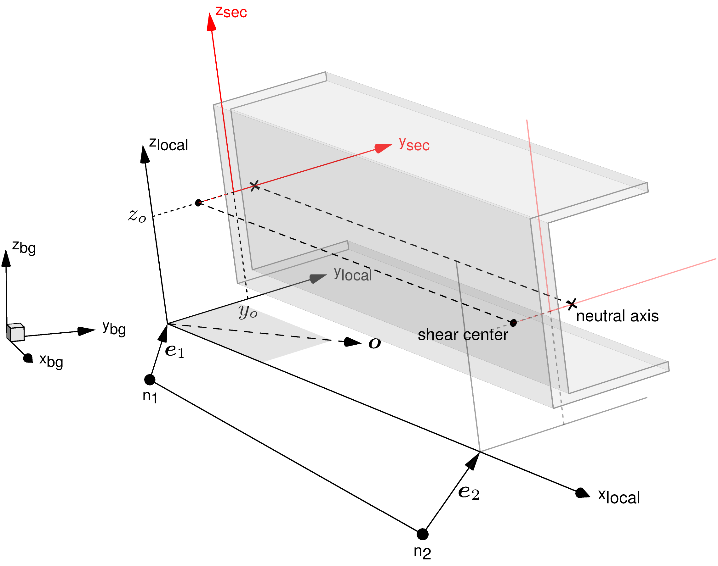
branch_orientation specifies the orientation of all node
coordinates of the current branch/mesh (or the default branch 1) with
respect to the global Cartesian coordinate system. If no
branch_orientation is specified, the node coordinates are
expressed in the global coordinate system.
MDL Specification
branch_orientation
    [base u1 u2 u3 v1 v2 v3]
    [rotate axis x|y|z angle a]
    [translate tx ty tz ]
end
Parameters
baseu1u2u3v1v2v3
Calculate the base from the vectors \(u\) and \(v\) as
follows: \(u\) defines the branch base \(e_1\), \(u
\times v\) defines the branch base \(e_3\), and \(e_3
\times u\) defines the branch base \(e_2\).
rotateaxisx|y|zanglea
Rotate the current branch base about the x, y, or z axis by a
degrees, and according to the right-hand rule. Successive rotations
can be specified.
rotateaxisu1u2u3anglea
Rotate the current branch base about the axis defined by the vector
u by a degrees, and according to the right-hand
rule. Successive rotations can be specified.
translatetxtytz
Translate the current branch by tx in the x-direction, ty
in the y-direction, and tz in the z-direction. All values are
float values. The default translation is 0.0 in all three
directions.
Example
The current branch is translated by x=50, y=20 and rotated by 30
degrees about the z-axis:
case specifies all ingredients needed for the analysis case
identified by IDENT (positive int), in particular the boundary
conditions, the initial conditions, and the solution strategy
parameters.
To activate the analysis case in the solver, a case must be specified
with they the case parameters of the adir command.
MDL Specification
case IDENT
   parameters
end
Parameters
The attributes enumerated in this section pertain to most types of
analyses and concern the specification of initial conditions sets,
boundary condition sets, and constraint sets. Solver-specific
attributes are explained in the Solvers.
analysisT
Optional type of analysis for the present analysis case. If
several cases are specified in an MDL input file the analysis
type must be the same of all cases. The string T is one of
linear
Linear static (or stationary) analysis, see
Linear Static Solver. This is the default analysis
type (new from version 4.5.3. Previous versions MUST
specify the analysis type!).
Optional type of implementation to use when solving the system.
This setting overwrites the solver class to use for the computation
implied by the analysis above.
The string TI is one of
slsbench
A solver to set up a static linear system without actually solving
it, for benchmarking purposes.
Specifies a component to be included in the current analysis
case. Components are extensions to b2000++. They implement
specific natural boundary conditions, essential boundary
conditions, initial conditions, or sets of constraints. The
component and type parameters are used to identify the
component, while the argument parameter is given to the
component at the start of the analysis (stage). sfactor and
sfunction are explained below.
dof_initIDENT
dof_init specifies the initial DOF conditions identified by
IDENT (e.g. displacements or temperatures). Note that only
one single dof_init identifier can be specified for the
current case.
rate_initIDENT(ordofdot_initIDENT)
`rate_init specifies the first time derivatives of the initial DOF
conditions (i.e. velocities) identified by IDENT. Note that
only one single rate_init identifier can be specified for the
current case.
acceleration_initIDENT
`acceleration_init specifies the second time derivatives of the
initial DOF conditions (i.e. accelerations) identified by IDENT.
Note that only one single acceleration_init identifier can be
specified for the current case.
ebcIDENT[sfactorS|sfunction"EXPRESSION"]
Includes the essential boundary conditions
identified by IDENT. Note that essential boundary conditions are
not cumulative, i.e. if several essential boundary condition sets
are specified, all values of common degrees-of-freedom must be
equal. sfactor and sfunction are explained below.
field_transferIDENT
Includes the field_transfer set identified by
IDENT. The field_transfer set with an IDENT of 0 is
automatically added to all analysis cases.
Alternatively, several or all field_transfer sets may be
specified:
field_transfer 123
field_transfer all
The accuracy of the calculated solution cannot always be ensured
when field_transfer conditions are active. Therefore, a
contraint method other thatn the default reduction methods
must be specified, Linear and Nonlinear Constraint Control.
joinIDENT
Includes the join set identified by IDENT in the current
analysis case. Note that a join set with an identifier of 0 is
automatically added to all analysis cases.
gradientsVALUEKEYSELECTION
Controls the computation of the gradients (strains, stresses,
heat transfer, etc.) for the current case. Specifying a positive
integer value (e.g. 1) for VALUE means yes. A value of 0
means no. Default is 0.
Note
The KEY and SELECTION fields are only available
for the default branch i.e. 1. If multiple branches are
specified, leave KEY and SELECTION field empty.
KEY can be used to specify which elements to compute and store
gradients for. If nothing specified, default behaviour is all
elements. e.g. Gradients1 computes and stores gradients for
all elements. KEY could be elements, allelements,
elementlist and elementset.
Aside from allelements which does not need any SELECTION
specifier, the other keys need element specification. For
elements, the element list could be provided in the SELECTION
field such as [e_1e_2e_3] where e_i is the external element
id from the .mdl input file. For elementlist and
elementset, the corresponding NAME needs to be specified in
the SELECTION field.
gradients_onlyyes|no
Specifies whether only gradients (and reaction forces) should be
computed, while the solution vector is defined solely by the the
initial conditions and the boundary conditions. Default is
no.
lincIDENT
Includes the :ref:linearconstraints<mdl.linc>`setidentifiedby``IDENT in the current analysis case. Note that a
linc set with an identifier of 0 is automatically added to
all analysis cases.
nbcIDENT[sfactorS|sfunction"EXPRESSION"]
Includes the natural boundary conditions
set identified by IDENT in the current analysis case. Natural
boundary conditions are cumulative, i.e. if several natural
boundary condition sets are specified the resulting natural
boundary condition for IDENT is the sum of all natural boundary
condition sets multiplied by their respective
scaling. sfactor and sfunction are explained below.
rcfo_restrictWHAT
Specifies to which nodes the calculation of reaction forces
shall be restricted in post-processing. This parameter is
ignored by the b2000++ solvers. If not specified, the relevant
Simples functions or
baspl++ will loop over all nodes of the model to
calculate the reaction forces. WHAT is one of:
epatchIDENTP1-P8|E1-E12|F1-F6|B
epatchIDENTPX|EX|FX|B
Selects nodes from an epatch. Individual patch vertex
nodes are specified with the strings P1 to P8. Patch
edge nodes are specified with the strings E1 to
E12. Patch face nodes are specified with the strings
F1 to F6. Patch body nodes of the whole patch body
are specified with the string B.
nodesetNAME
Specifies the name of the node set
to be included.
Override the automatically selected sparse solver type by
prescribing a specific sparse linear solver type (string). See
B2000++ Sparse Linear Equation Solvers.
stageIDENT[sfactorS|sfunction"EXPRESSION"]
Includes an analysis adir identified by IDENT. One or
more stages can be defined for the current case. If more than one
stage is specified, the solver will solve for one stage after the
other in the order stages have been listed. If one or more
stage parameters are specified for a given analysis case, no
other may be specified for that particular case.
subcaseparameters...end
Defines a subcase of the current case. The subcase will inherit
all case options, specifically the essential boundary
conditons. In the present version only nbc case parameters
also apply to subcase.
temperaturesIDENT[sfactorS|sfunction"EXPRESSION"]
Includes the temperatures set identified by IDENT to be
included for thermal stress analysis. sfactor and
sfunction are explained below.
title'TEXT'
Optional title describing the case.
sfactor and sfunction
In linear analysis, the optional parameter sfactor specifies a
scale factor S by which the set is multiplied, the default value
being 1.0.
In nonlinear direct analysis and in incremental analysis, the set is
scaled by the load factor (static analysis) or by the time (dynamic
analysis). The optional parameter sfactor specifies an additional
scale factor S by which the set is multiplied, the default value
being 1.0. Alternatively, the optional parameter sfunction
specifies a function which is being evaluated at each load or time
increment and by which the set is multiplied.
Per-Stage Commands in Multi-stage analysis
During nonlinear analysis, it is often necessary to split the loading
path into a series of stages. In this example, case 3 is executed,
which consists of two stages (defined by stages 1 and 2). To ensure
convergence of the nonlinear solver in the presence of buckling
(load-controlled by default), artificial damping is performed to
stabilize the problem.
stage 1
  ebc                   1
  nbc                   1
end

stage 2
  ebc                   2
  step_size_init        0.05
  step_size_max         0.05
end

case 3
  analysis              nonlinear
  residue_function_type artificial_damping
  stage                 1
  stage                 2
end

adir
  case 3
end
The b2000++ solver initializes many of its internal procedures and
data structures on a per-case basis, not on a per-stage basis. The
commands for the various methods are interpreted only during this
initialization phase. Specification of commands like
residue_function_type in a case defining stages will be ignored.
Instead, they must be placed in the definition of another case (case
3 in the above example). Consequently, residue_function_type will
be active for both stages.
On the other hand, commands controlling the step size and the
tolerances for the residual, solution, etc., can be defined in a case
containing stage specifications.
Components
A component can implement a weakly-coupled fully-nonlinear
aero-elastic tool-chain. In this case, the values taken by the
component are the current (nodal) displacements (calculated by
b2000++), and the values returned by the component are the (nodal)
forces. To this end, at each Newton iteration (or each n-th Newton
iteration), the component invokes the spatial coupling tool, the CFD
mesh deformation tool, the CFD solver, and again the spatial coupling
tool.
dof_init defines initial conditions, i.e DOF fields (such as
displacements or temperatures). The dynamic (transient) or non-stationary
solver will include initial DOF fields at time t = 0. If no initial
conditions are specified the solver will assume all initial conditions to
be 0. A dof_init set is identified by IDENT (non-negative int).
IDENT is the number which is referenced by the dof_init options of
case. Sets with an identifier of 0 will be active for all analysis
cases. To set initial velocities or accelerations, see rate_init or
acceleration_init, respectively.
MDL Specification
dof_init IDENT | rate_init IDENT | acceleration_init IDENT
   value V
   DOFLIST...
   NODESPECIFICATION...
   ...
end
Values and Degrees-of-Freedom
valueV
Specifies the value V (float) to be assigned to subsequently
specified nodes. The value is assigned to a subsequently defined
DOF’s!
dofI1 or dof[I1I2...]
Specifies the DOF(s) identifier(s) for which the value v will
be assigned. DOF identifiers can be integers (DOF numbers are
1,2,3,…) or strings:
During stress analysis, UX, UY, and UZ represent
the displacement in the x-, y-, and z-direction, respectively.
During stress analysis, RX, RY, and RZ represent
the rotation (in radians) about the x-, y-, and z-axes,
respectively.
During heat analysis, T means the temperature.
The degrees-of-freedom that are present at a given node depend
on the elements to which this node is connected. Specifying a
value for a degree-of-freedom that does not exist will have no
effect.
Node Specification
allnodes
Assign the initial conditions to all defined nodes of the current
branch.
branchBR
Specifies the external branch number BR. Default is 1.
epatchIDENTP1-P8|E1-E12|F1-F6|B
Includes nodes generated with an existing epatch identified
by IDENT. Individual patch vertex nodes are specified with
P1 to P8. Patch edge nodes are specified with E1 to
E12.Patch face nodes are specified with F1 to F6. The
patch body nodes are specified with B.
nodesN or nodes[N1N2...]
Explicitly specifies a nodes identifiers (of the current branch)
to which the initial conditions will be assigned.
nodesetNAME
Specifies the name of the node set
which the initial conditions will be assigned.
The ebc command specifies essential boundary conditions, such as
single-point constraints, and assigns them to variables, such as
displacements in case of solid mechanics, temperatures in case of heat
transfer analysis, etc. An``ebc`` set is identified by the identifier
IDENT (non-negative int). IDENT is the number which is
referenced by the ebc parameter of the case definition. Sets
with an identifier of 0 will be active for all analysis cases.
Essential boundary conditions can be specified for nodes or, in case
where elements have internal degrees-of-freedom, for elements.
MDL Specification
ebc IDENT [system S] [title T]
parameters
node-specifications
end
Parameters
systemBRANCH|LOCAL
Specifies the reference frame in which the conditions are
formulated. The default reference frame is LOCAL.
BRANCH means that the constraints are formulated with respect
to the branch-global reference frame, irrespective of node-local
reference frames at any node. LOCAL means that the
constraints are applied to the node-local reference frame(s)
where defined, and to the branch-global reference frame
otherwise.
title"TEXT"
Specifies an optional title for the ebc set.
dofI or dof[I1I2...]
Specifies the DOF(s) identifier(s) for which the value V will
be assigned. DOF identifiers can be integers (DOF numbers are
1,2,3,…) or strings:
During stress analysis, UX, UY, and UZ represent
the displacement in the x-, y-, and z-direction, respectively.
During stress analysis, RX, RY, and RZ represent
the rotation (in radians) about the x-, y-, and z-axes,
respectively.
During heat analysis, T means the temperature.
The degrees-of-freedom that are present at a given node depend
on the elements to which this node is connected. Specifying a
value for a degree-of-freedom that does not exist will have no
effect.
valueV
Specifies the value V (float) to be assigned to subsequently
specified nodes. The value is assigned to a subsequently defined
DOF’s!
Node Specification
allnodes or allelements
Assign the initial conditions to all defined nodes of the current
branch.
branchBR
Specifies the external branch number BR. Default is 1.
epatchIDENTP1-P8|E1-E12|F1-F6|B
Includes nodes generated with an existing epatch identified
by IDENT (node specification only). Individual patch vertex
nodes are specified with P1 to P8. Patch edge nodes are
specified with E1 to E12.Patch face nodes are specified
with F1 to F6. The patch body nodes are specified with
B.
nodesN or nodes[N1N2...]
Specifies node identifiers (of the current branch) to which the
initial conditions will be assigned.
Specify the ebc set 123: For the mesh node 1, set all 6 DOF’s
to 0. For the mesh nodes 9,10,11,12, set the z-rotation to 0, and for
mesh node 9, the y-displacement 2 to 0.12.
ebc 123
  value 0.   dof [UX UY UZ RX RY RZ] nodes 1
  value 0.   dof RZ                  nodes 9
  value 0.12 dof UY                  nodes [9 10 11 12]
end
The ebc set must then be activated by referencing it in one of the
cases to be computed. Example:
case 20
   ...
   ebc 123
   ...
end
Element-internal Degrees-of-Freedom
Some element formulations involve internal degrees-of-freedom. With
the ebc command it is possible to prescribe values to these DOFs,
e.g for debugging purposes. With elements, the individual
degrees-of-freedom are identified by numbers, starting from
1.
For example the shell element Q4.S.MITC.E4 is an
enhanced-assumed-strain element with 4 internal degrees-of-freedom.
Locking them for all elements is done as follows:
value 0 dof [1/4] allelements
Additional information
To activate essential boundary condition sets, add the required
essential boundary condition set identifiers to the case
definition.
Node-local coordinate systems can be defined with the
transformations command. The b2000++ coordinate systems are
described in the programming manual.
Natural boundary conditions can be defined with the nbc
command.
Please read the additional notes in the description of the
join command for information on branch connectivity.
edgeset defines an element edge set list containing pairs
(IDENT, EX) of a specific branch. IDENT is the external
element identifier and EX the edge identifier (E1, E2,
…). The list is identified by the NAME of the set (a string not
exceeding 40 characters). Note hat edge sets are not defined for
special elements, such as RBE.
MDL Specification
edgeset NAME sorted|unsorted
    branch BR
    EX
    edgeset NAME1
    epatch IDENT
    n1 n2 ...
end
Parameters
sorted|unsorted
sorted creates an ordered set with all duplicates
removed. unsorted adds nodes as they are specified. Default is
unsorted. sorted or unsorted must be specified
directly after NAME and before any other parameter.
branchBR
Specifies the branch number to which subsequently defined element
identifiers will be assigned. The default branch is 1. BR
remains active until a new branch is specified or end is
encountered.
EX Specifies the edge number x (1.:12). All subsequently listed
elements will inherit this edge number. The default element edge
identifier is E1. Generic Elements describes the
element edge definitions for relevant elements.
edgesetIDENT
Copies all edge identifiers found in an existing edge set IDENT
to the current face set.
epatchIDENTE1...E12
Copies all edge identifiers of the edge Ex of the existing
epatch with identifier IDENT.
N1N2...
Specifies a list of external element identifiers. The current edge
number will be assigned to these element identifiers until a new
edge number is specified (if any).
Examples
Specify the edge set edge1 containing the edge identifiers of the
edge of a plate patch consisting of 2 by 2 Q4 elements for (default)
branch 1.
epatch generates simple one-dimensional, two-dimensional, and
three-dimensional regular meshes. For one-dimensional patches,
straight or arc lines can be modeled. For two-dimensional patches,
four-sided surfaces described by analytical functions can be modeled,
creating Q shell-type elements. For three dimensional patches, cubes
described by analytical functions can be modeled, creating HE
solid-type elements. In addition to nodes end elements, epatch
also generates lists containing vertex, edge, face, and body node
indices and element indices, thus facilitating the generation of
boundary conditions. Note, however, that the epatch command is by
no means a substitute to any modeling and meshing software.
Any number of element patches can be generated within the same branch
definition, provided that the patch boundary nodes match, i.e. nodes
are not merged automatically if several element patches are generated
in one and the same branch. Thus, it is often easier to generate one
element patch per branch and connect the branches with the automatic
option of the join command.
Element patches generate elements as follows (see also the figure below
for the definition of i, j, and k): For all elements in the k-direction,
for all elements in the j-direction, generate elements in the
i-direction, incrementing the element number by one.
Note that the default initial element number and the default initial
node number are both set to the highest internal element or node number
plus 1, defined so far for the current branch. Internal element and node
numbers start with 1. If patches and element and node definitions with
the elements and nodes commands are defined within the same
branch please consider making use the element start index
start_element_id or the node start index start_node_id options
to avoid conflicts with external element or node numbers defined by the
elements or nodes commands and the epatch element and node
generation, which generates internal node numbers.
A patch is meshed independently of any other patches, and when
defining multiple patches, the coinciding nodes of adjacent patches
will not be connected. Coinciding nodes can be connected by means of
the join (using the automatic option).
Two-dimensional element patch definition: Patch edges. The patch face
is f7 or mid_surface.
Three-dimensional element patch definitions: Patch edges.
Two- and three-dimensional element patch definitions: Patch faces.
Parameters
eltypeT
Specifies the element type T of the patch. For 1D patches
elements of type B, C, L and R are allowed. For 2D patches elements
of type T and Q are allowed. For 3D patches, element types HE and -
to some extent - TE are allowed. The element type may only be
specified once for one and the same patch.
geometryGTYPE
Specifies the geometry type of the patch to be generated. The
following geometry types GTYPE and their parameters can be
defined:
ARCH
Creates a line mesh of beam/rod/cable/line elements along a
circular arch that is defined in the branch x-y plane and
with the origin of the circular segment at (0,0,0). Required
meshing parameters are the number of elements ne1 (int),
the radius R (float), the start angle angle1 (float),
and the end angle angle2``(float).Theoptionalparameter``open (YES``|``NO) applies only in case where the
segment makes a full circle. By default, the coinciding nodes
are merged. Setting open to YES retains the duplicate
nodes.
cylinder
Specifies a cylindrical shell segment. The generated segment
is defined in the branch x-y plane, with the origin of the
circular segment at (0,0,0), a radius r, and with the
angles phi1 (start angle) and phi2 (end angle)
rotating around the z-axis. The axial direction is in the
branch z-direction. Required meshing parameters are the
number of elements ne1 in the circumferential
i-direction and the number of elements ne2 in the axial
j-direction. The thickness parameter is element type
dependent.
cube
Creates an isoparametric solid mesh of a cube defined by the 8
corner nodes p1 to p8. Required meshing parameters are
the number of elements ne1 in the i-direction, the number
of elements ne2 in the j-direction, and the number of
elements ne3 in the k-direction. All other parameters are
element type dependent.
line
Creates a straight line mesh of beam/rod/cable/line elements
extending from point p1 to point p2, with an optional
area or thickness t. Required meshing parameters are the
number of elements ne1 in the i-direction. All other
parameters are element type dependent.
plate
Generates an isoparametric rectangular plate mesh defined by
the four corner nodes p1 to p4. The plate has a
optional uniform thickness t. Required meshing parameters
are the number of elements ne1 in the plate i-direction
and the number of elements ne2 in the plate
j-direction. All other parameters are element type
dependent. The thickness parameter is element type
dependent.
ring
Specifies a 2D shell element mesh of a ring. The ring is
defined in the branch x-y plane, with the origin of the
circular segment at (0,0,0) and with the following keywords:
phi1 (start angle) and phi2 (end angle) rotating
around the z-axis define the angles. The ring segment has an
inner radius radius1 and an outer radius radius2.
Required meshing parameters are the number of elements ne1
in the circumferential (i-) direction and the number of
elements ne2 in the radial (j-) direction. The
thickness parameter is element type dependent. The
open parameter applies only in case where the segment
makes a full circle. By default, the coinciding nodes are
merged. Setting open to yes retains the duplicate
nodes.
tube
Specifies a solid mesh of a tube. The tube section is defined
in the branch x-y plane, with the origin of the circular
segment at (0,0,0) and with the following keywords: The angles
phi1 (start angle) and phi2 (end angle) rotating around
the z-axis defined the angles. The tube has an inner radius
radius1 and an outer radius radius2. The length of the
tube is defined by the length. Required meshing parameters
are and the number of elements ne1 in the circumferential
(i-) direction, the number of elements ne2 in the radial
(j-) direction, and the number of elements ne3 in the
global z (k-) direction. The open parameter applies only in
case where the segment makes a full circle. By default, the
coinciding nodes are merged. Setting open to yes
retains the duplicate nodes.
localNONE|EDGES|ALL
Specifies if the generated nodes will be assigned a node-local DOF
reference coordinate system (see transformations and
nodes). The node-local coordinate system is generated
according to the geometry type. edges generates local
reference coordinate systems for all nodes placed on patch edges.
ALL generates local reference coordinate systems for all
nodes.
ne1N
Specifies the number of elements in regular patch in the logical
i-direction, see figure above (required for all patches).
ne2N
Specifies the number of elements in regular patch in the logical
j-direction, see figure above (required for 2D and 3D patches).
ne3N
Specifies the number of elements in regular patch in the logical
k-direction, see figure above (required for 3D patches).
orientationUXUYUZVXVYVZ
Defines a local base by which all epatch nodes are rotated (refer to
the section on orientation below for more details).
start_element_idIDENT
Element identifier of first element generated. All subsequent
elements are generated by incrementing the element identifier by 1,
first in the i-direction, then in the j-direction, and, finally, in
the k-direction. The default value is 1.
start_node_idIDENT
Node identifier of first node generated. All subsequent nodes are
generated by incrementing the node identifier by 1, first in the
i-direction, then in the j-direction, and, finally, in the
k-direction. The default value is 1.
translationTXTYTZ
Translates the patch in the branch global x-, y- and z-direction.
All other keywords are element-dependent.
The orientation directive allows to change the orientation of any
patch. This may be useful in the case of cylindrical patches which
have a default orientation (the cylindrical axis is aligned with the
branch-global z-direction).
The following directives can be used to modify the orientation:
baseu1u2u3v1v2v3
Calculate the base from the vectors u and v as follows: u defines the
patch base e1, u x v defines the patch base e3, and
e3 x u defines the patch base e2.
rotateaxisX|Y|ZangleA
Rotate the current patch base about the X, Y, or Z axis by A degrees,
and according to the right-hand rule. Successive rotations can be
specified.
rotateaxisU1U2U3angleA
Rotate the current patch base about the axis defined by the vector
u1 u2 u3, by a degrees, and according to
the right-hand rule. Successive rotations can be specified.
translateTYTYTZ
Translate the current patch by TX in the x-direction, TY in the
y-direction, and TZ in the z-direction. TX, TY, and TZ are float
values. The default translation is 0.0 in all three directions.
All element attributes are element type dependent and can be consulted
in the elements sections of the user manual.
Examples
Generate a cylindrical panel mesh with a 90 degree opening, starting
at phi=0. The panel has a radius of 1., a thickness of 0.002, and a
length of 1. All nodes shall have a local cylindrical coordinate
system (r, phi, z). The panel is meshed with Q9 shell elements.
Generate a cylindrical panel mesh identical to the one in the
preceding example, i.e with a 90 degree opening, starting at
phi=0. The panel has a radius of 1., a thickness of 0.002, and a
length of 1. All nodes shall have a local cylindrical coordinate
system (r, phi, z). The panel is meshed with Q9 shell elements. The
cylinder shall be rotated by +90 degrees around the y-axis: This is
achieved by defining local base vectors with the orientation
parameter.
Generate a cylindrical panel mesh with a 90 degree opening, starting at
phi=0. The panel has a radius of 1., a thickness of 0.002, and a length
of 1. All nodes shall have a local cylindrical coordinate system (r,
phi, z). The panel is meshed with 10 by 5 Q8 shell elements.
elements defines mesh elements on a one by one element basis. To
generate elements (and nodes) for various simple geometries, make use
of the epatch command.
An element is defined by the element type, the parameters describing
the element properties and the external element identifier IDENT
and the element node connectivity list.
MDL Specification
elements
   eltype ET
   parameters
   IDENT N1 N2 N3 ...
   ...
end
Parameters
Except for the element type and the node connectivity definition
below, the required and optional element parameters depend on the
element type and are explained in the specific element sections.
eltypeET
Specifies the element type (required if element property
parameters are defined). All elements defined thereafter will be
of type ET until a new ET is specified. eltype always
invalidates all required attributes and resets all optional
attributes to their default values.
It is possible to initially specify a dummy element type when
defining the element connectivities and to change it later. This
can be useful when the mesh and the elementsets are created by an external program, or when
the mesh definition shall be independent of the operator. In this
case, the correct element type and the element attributes need to
be set at a later stage (see below). The following dummy element
types are available:
P for point elements.
L2 and L3 for linear and quadratic line elements,
respectively.
T3 and T6 for linear and quadratic triangular elements,
respectively.
Q4, Q8, and Q9 for quadrilateral elements.
TE4 and TE10 for linear and quadratic tetrahedral elements,
respectively.
PR6 and PR15 for linear and quadratic prismatic elements,
respectively.
HE8, HE20, and HE27 for hexahedral elements.
IDENTN1N2N3...
Specify a single element with external element identifier IDENT
and external element node identifiers N1N2N3... defining the
element node connectivity. See the specific elements
sections for a definition of the element node connectivity.
IDENT[ni|nodesetNAME...]
Defines an element with external identifier IDENT and a variable
number of node identifiers specified explicitly or by
referencing. nodeset includes all nodes of a nodeset in
the current list.
Examples
Define two four node quadrilateral shell element with the external
numbers 10001 and 10002, having a constant shell thickness of 1.3 (for
the element parameter see Shell Elements):
For elements with a potentially large number of nodes, such as
RBE elements, the use of one or several
nodesets (not node lists!) may be convenient:
eltype RBE
   1001  [100001  nodeset left]
   1002  [100002  nodeset right]
   1003  [100002  nodeset front  nodeset back]
end
Specify 4 elements: Two four node quadrilateral shell elements with a
constant thickness of 1.3, and two elements of the same element type
with a constant thickness of 1.5:
elementset defines a named list NAME containing external
element identifiers EID1, EID2, … of a single
branch. NAME is a string not exceeding 40 characters and must be
unique within the model. Element identifiers EID are positive int
values. Element sets are not linked to element types and can be
specified for all element types.
MDL Specification
elementset NAME sorted|unsorted
    branch BR
    elementset NAME1
    epatch IDENT
    <element identifier specification list>
    EID1 EID2 ...
end
Parameters
sorted|unsorted
sorted creates an ordered set with all duplicates
removed. unsorted adds nodes as they are specified. Default is
unsorted. sorted or unsorted must be specified
directly after NAME and before all specifying element
identifiers.
branchBR
Specifies the branch number to which subsequently defined element
identifiers will be assigned. The default branch is 1. BR
remains active until a new branch is specified or end
is encountered.
elementsetNAME1
Copies all element identifiers found in an existing element set
NAME1 to the current set.
epatchIDENT
Copies all elements identifiers defined for the existing
epatch with identifier IDENT to the current set.
<elementidentifierspecificationlist>
List of external element identifiers specified one by one and/or
sequences from/to/step.
Note
Duplicates in the list are ignored when total volume, total mass,
and the center of mass of an element set are computed.
faceset defines a list assigning face number to elements, creating
pairs (elementid, faceid) of a specific branch. elementid
is the external element identifier and FX the face identifier (see
below). The list is identified by the NAME of the set (a string
not exceeding 40 characters). Note hat face sets are not defined for
wire (beam, rods) elements nor for special elements, such as RBE
elements.
MDL Specification
faceset NAME sorted|unsorted
   branch BR
   Fx
   faceset NAME
   epatch IDENT
   N1 N2 ...
   ...
end
Parameters
sorted|unsorted
sorted creates an ordered set with all duplicates
removed. unsorted adds nodes as they are specified. Default is
unsorted. sorted or unsorted must be specified
directly after NAME and before any other parameter.
branchBR
Specifies the branch number to which subsequently defined element
identifiers will be assigned. The default branch is 1. BR
remains active until a new branch is specified or end is
encountered.
Fx
Specifies the face number x (1..7). All subsequently listed
elements will inherit this face number. The default element face
number is 1. Chapter Generic Elements describes the element face
definitions for relevant elements.
facesetNAME
Copies all face identifiers found in an existing face set NAME
to the current face set.
epatchIDENTF1|F2|F3|F4|F5|F6
Copies all face identifiers of the face Fx of the existing
epatch with identifier IDENT.
N1N2...
Specifies a list of external element identifiers. The current face
number will be assigned to these element identifiers until a new
face number is specified (if any).
Examples
Specify the face set surface1 containing the face identifiers of the
element faces (face F1) of a plate patch consisting of 2 by 2 Q4
elements 1, 2, 3, and 4 of (default) branch 1:
field_transfer specifies coupling conditions between two adjacent
but in general incompatible surface meshes. In stress analysis, it
represents a kinematic coupling condition. A typical application is
global-local analysis with shell-to-solid, shell-to-shell, or
solid-to-solid coupling. Another application is skin-stiffened
structures with independent meshes for skin, stringers, frames,
etc. In heat analysis, it couples the temperature fields of the two
adjacent surfaces.
The coupling is a weighted-residual method based on the \(L_{2}\)
norm of the difference of the interpolated fields at the surfaces.
A field_transfer condition must be activated in the case
command. If the identifier IDENT is 0, the coupling condition will
be automatically added to all analysis cases. It is required to
specify a constraint method other than the default reduction
method for which the accuracy of the calculated solution cannot be
guaranteed when field_transfer conditions are active. The
constraint method is defined in the case block, see
section Linear and Nonlinear Constraint Control.
The surfaces to be coupled are defined by interfacei where i is
either 1 or 2. An arbitrary number of surface sets faceset
may be added to each interface.
When the analysis is started, a common-refined mesh consisting of
surface triangles is created from the intersection of the two coupling
interfaces, according to the element face shapes. In the case of flat
geometries, this common-refined mesh coincides exactly with both surface
meshes. In the case of curved geometries, the common-refined mesh
approximates both surface meshes. The approximation error can be reduced
by setting num_subdivision to a positive value. In this case, the
surface mesh of the respective interface will be n-times recursively
subdivided.
The calculation of the interpolated field at the interfaces is conducted
using the shape functions of the involved elements. Integration over the
triangles of the common-refined mesh is carried out according to the
element interpolation order(s). This way, the coupling is accurate for
low-order as well as for high-order elements.
The transfer directive specifies the type of field to be transferred
and on which interface i the residuum shall be minimized.
join command specifies equality between the DOF’s of nodes joined
together. join is identified by IDENT (positive or zero value
int). IDENT is the identifier referenced by the join option of
case. join sets with an identifier of 0 will be activated for all
analysis cases.
The join command is required if more than one branch (mesh) is
defined and the branches (meshes) are to be connected or if nodes of
the same branch (mesh) are to be connected explicitly. Note that the
same effect can be obtained by specifying linear constraints, see
linc, although on a DOF by DOF base.
join must be follow all nodes and elements specifications of an MDL file.
MDL Specification
join IDENT
   parameters
   coupling conditions...
end
Parameters
deltaV
Specifies the threshold value V in the global x-, y- and
z-directions for comparing nodes (relevant for the automatic
parameter only). This option must be issued before automatic
in order to take effect. If not specified, the threshold value
will be computed as a function of the bounding box.
automatic
Establishes the node connectivity automatically by comparing node
positions. The nodes are transformed to the global-global
coordinate system. If the nodes are close enough (see delta
parameter) they will be linked. Note that the node and
dof coupling commands may not be specified if automatic is
selected. No other parameter can be specified after the
``automatic`` option.
Coupling Conditions Specification
nodeBR1N1BR2N2
Generates links node-wise. Node N1 of branch BR1 is
linked to node N2 of branch BR2. The automatic
command may not be specified if node is selected. Branch and
node numbers are external.
dofBR1N1DOF1BR2N2DOF2
Generates links between degrees-of-freedom. The degree-of-freedom
DOF1 of node N1 of branch`` BR1`` is connected to the
degree-of-freedom DOF2 of node N2 of branch
BR2. Branch and node numbers are external. degree-of-freedom
numbers are positive integers.
Examples
The most common use of join is:
join 0
   automatic
end
Explicit joining of nodes: Connect node 3 t node 33, both in branch
(mesh) 1.
join 0
   node 1 3 1 33
end
Additional Notes
Master nodes are automatically determined as follows: The node belonging
to the lower branch number in the link list becomes the master node.
For automatically computed link lists, the node lists are compared
branch-wise and in ascending order (internal branch numbering). The
first encountered node that matches another node in the list becomes the
master node. The matching criteria are defined by a cube of size (delta,
delta, delta) constructed around the node.
linc IDENT [tol_drop V]
   equation1
   equation2
   ...
end
Description
The linc command specifies one or more linear constraint equations.
Linear constraint equations and their terms can be specified in any
order. There are no a priori restrictions on the nodes and
degrees-of-freedom that may be specified in linear constraints, since
b2000++ does not distinguish between master and slave nodes.
A linc set is identified by IDENT (positive or zero value
int). IDENT is the number which is referenced by the linc
option of the case command.
Note
Sets with an IDENT of 0 will be active for all analysis cases.
The constraint equations are of the form
\[c_{i} u_{i} + c_{0} = 0, i=1,n\]
where the coefficients \(c_{i}\) pertain to the dof’s of the global
equation system.
In case nodes are to be explicitly connected it is preferable to make
use of the join command, because it connects all DOF’s and it
also ensures that node types are processed properly.
Parameters
tol_dropV
Sets the value for the drop tolerance. Default is 1e-4. Any term
of subsequently specified equations with an absolute weight below
the drop tolerance will be ignored.
Equations Specification
equationNCC_0B1N1DOF1C1...BnNnDOFnCn
Specifies a complete constraint equation with n terms as listed
above. Each term is described by the external branch number
Bi, the external node number Ni, the degree-of-freedom
DOFi relating to node Ni, and the constant Ci.
Additional Information
Depending on how linear constraints are enforced (see
Linear and Nonlinear Constraint Control), the system of linear equations may
need to be modified to ensure a well conditioned global stiffness
matrix. Automatically generated linear constraint equations may
contain very small weights, which my result in a poorly conditioned
global stiffness matrix. When using the default reduction method for
linear constraints, it is recommended to set tol_drop to a
sufficiently large value.
If weights below 1e-4 are specified but the drop tolerance is smaller,
the b2000++ input processor b2ip++ will print a warning.
To check whether the calculated solution is accurate, an error
analysis on the matrix factorization and back-substitution process can
be conducted by specifying the b2000++ command-line option
b2000++-l'debug of linear_algebra'DBNAME
when executing b2000++.
Example
Establish a rigid link between displacements in the x-direction (dof 1)
by coupling node 23 of branch 1 to node 45 of branch 4:
material specifies the physical properties of an element material.
Element materials are identified by a positive integer IDENT,
which is then referenced by the elements (see
elements). Element material definition is branch-independent,
i.e. the element material identifiers IDENT are global. The
material command creates the data set MATERIAL.id. The
detailed material specification is described in the materials section.
The nbc command specifies natural boundary conditions (NBC)
applied to the DOF’s of specific nodes. Natural boundary conditions
will be part of the right-hand side of the problem to be solved.
An nbc set is identified by the identifier IDENT (non-negative
int). IDENT is the number which is referenced by the nbc option
of the case definition. Sets with an identifier of 0 will be
active for all analysis cases.
An nbc is of a certain type (i.e. concentrated forces, line loads,
surface fractions, heat) and is specified either in the branch-global
reference frame, the node-local reference frame, the element edge or
face reference frame, or the deformed element edge or face reference
frame.
A natural boundary condition set is activated with the nbc option
of the case command.
The type concentrated_loads (the default) means that concentrated
loads (i.e. forces in stress analysis and heat in heat transfer
analysis) are assigned to degrees-of-freedom at individual nodes or
multiple nodes.
nbc IDENT [type concentrated_loads] [system S] [title T]
  value V
  dof list
  node specification...
  value V
  dof list
  node specification...
  ...
end
Parameters
The degrees-of-freedom that are present at a given node depend on the
elements to which this node is connected. Specifying a value for a
degree-of-freedom that does not exist will have no effect.
valueV
Specify the magnitude of a single value (float) i.e concentrated
load or heat). This value is then assigned to one or several
degrees-of-freedom by means of the directive dof. The couple
(value, degrees-of-freedom) is then assigned to individual nodes
or collections of nodes. You can only specify a single value
V.
dofI1dof[I1I2...]
The directive dof is followed by a list which identifies the
degrees-of-freedom:
In stress analysis, FX, FY, and FZ represent a
force in the x-, y-, and z-direction, respectively.
In stress analysis, MX, MY, and MZ represent a
moment about the x-, y-, and z-axes, respectively.
In heat analysis, Q means the rate of heat flow (power).
Node Specification
allnodes
Assign the concentrated loads to all defined nodes of the current
branch.
branchBR
Specifies the external branch number BR (positive
int). Default is 1.
epatchIDENTp1-p8|e1-e12|f1-f6|b
Applies to conditions to node lists of an existing
epatch identified by IDENT. Individual patch vertex
nodes are specified with p1 to p8. The collection of
nodes that are located at a patch edge are specified with
e1 to e12. The collection of nodes that are located at
a patch face are specified with f1 to f6. The
collection of nodes of the whole patch body are specified with
b.
nodesN or nodes[N1,N2...]
Apply the condition(s) to a node or a list of nodes.
nodesetNAME
Specifies the name of the node set to
which the concentrated loads will be assigned.
Examples
Set the force in the y-direction to 25.0 for mesh node 5. For mesh
nodes 9,10,11,12, set the moment in the y-direction to 60.0. Since
the default reference frame is node-local, the directions will be the
node-local directions if there are local coordinate system defined for
these nodes. Otherwise, the directions will be aligned with the branch
reference frame.
nbc 1
   value 25.0 dof FY nodes 5
   value 60.0 dof MY nodes [9 10 11 12]
end
Apply a concentrated force in z-direction to the center node (p5)
of a square plate meshed with the epatch command. Note: The center node
is defined only if the number of elements in the patch directions
(ne1 and ne2) are even!
Specifying typeline_loads means that the set consists of line
loads (force per unit length in stress analysis), which will be
integrated along the element edges during the analysis by the element
implementations. The element thickness is not taken into account.
Line loads are meaningful for shell elements (edges 1-4), 2D elements
(edges 1-4), and cable/rod and beam elements (edge 1). Irrespective of
the element type, line loads are specified with 3 components L1L2L3 (no square brackets!).
The default reference frame is local. For cable/rod elements and
beam elements, this means the element axis. Only the value of L1
is used while L2L3 will be ignored. For shell elements and 2D
elements, the edge-local reference frames will be used. They are
identical to the face-local reference frames of a corresponding solid
element:
L1 coincides with the edge direction.
L2 coincides with the element surface normal. For cable/rod
elements, beam elements, and 2D elements, L2 will be ignored.
L3 coincides with the outward-pointing face/edge normal. For
cable/rod and beam elements, L3 will be ignored.
The reference frame local_deformed is intended for geometrically
nonlinear stress analysis and otherwise identical to local. The
reference frame branch means that L1L2L3 is in the
branch-global x-, y-, and z-direction, respectively.
The default reference frame is local. If you want to generate
loads in the (branch) global system, you must specify
systembranch
before generating loads.
Warning
Generation of line loads (loads along a beam element or along an
edge of a shell or solid element) is bugged. The orientation of
the loads (system parameter) works correctly for systembranch only!
Parameters
edgeset"NAME"
Specifies the name of the edge set to
which the line loads will be assigned.
epatchIDENTe1-e12
Specifies an epatch edge to which the
line loads will be assigned.
Examples
A line load in y-direction is applied to the outer edge of a clamped
cantilever beam.
nbc IDENT type surface_tractions [system S] [title T]
   surface_tractions T1 T2 T3 | pressure P
   face specification...
   surface_tractions T1 T2 T3 | pressure P
   face specification...
   ...
end
Surface tractions are forces per unit area. They will be integrated
along the element faces during the analysis by the element
implementations. In case of 2D elements and shell elements, the
element thickness is taken into account.
Surface traction loads are meaningful for 3D elements (faces 1-6), shell
elements (edges 1-4 for the sides, face 5 for the lower surface, face 6
for the upper surface, and face 7 for the mid-surface), and 2D elements
(edges 1-4 for the sides). Surface traction load are specified with 3
components T1T2T3.
The default reference frame is local, which means that the
face-local reference frames of the initial configuration will be used
(see also Generic Elements):
T1 coincides with the edge direction in case of 2D and shell
elements.
T2 coincides with the element surface normal in case of 2D and
shell elements.
T3 coincides with the outward-pointing face normal.
The reference frame local_deformed is intended for geometrically
nonlinear stress analysis and otherwise identical to local. The
reference frame branch means that T1T2T3 is in the
branch-global x-, y-, and z-direction, respectively.
Specifies the name of the face set to
which the loads will be assigned.
epatchIDENTf1-f7
Specifies an epatch face to which the loads will
be assigned.
Examples
A uniform pressure is applied to the mid-surface of a square plate
which is simply-supported. The plate is generated with epatch
command. The nbc 2 is equivalent to the nbc set 1.
nbc IDENT type surface_flux [system S] [title T]
   surface_flux q
   face specification...
   surface_flux q
   face specification...
   ...
end
Surface fluxes are, for example, heat flux per unit area. They will be
integrated along the element faces during the analysis by the element
implementations.
Note
The surface_flux feature is currently only available for
hexahedral elements!
Surface flux loads are meaningful for 3D elements (faces 1-6), shell
elements (edges 1-4 for the sides, face 5 for the lower surface, face 6
for the upper surface, and face 7 for the mid-surface), and 2D elements
(edges 1-4 for the sides). Surface flux load is specified with 1 scalar
component q.
Parameters
faceset"NAME"
Specifies the name of the face set to
which the loads will be assigned.
epatchIDENTf1-f7
Specifies an epatch face to which the loads will
be assigned.
Examples
A heat flux is applied to face F4 of a hexahedral heat conduction
element. The rigid solid is generated with the epatch command.
nbc IDENT type body_loads [system S] [title T]
   body_loads FX FY FZ
   element specification...
   body_loads FX FY FZ
   element specification...
  ...
end
Generates body loads by integrating a force-per-unit-volume field over
the element volume.
Note
Do not make use of body loads in case you want to generate
loads due to the own mass of a structure under a gravity
(acceleration) field - refer to inertia loads.
Body loads can be applied to all 1D- 2D- and 3D elements, but they
should not be used with point-mass elements (the type
accelerations should be used instead).
Body loads are specified with 3 components F1F2F3, defined in
the branch-global reference frame (local reference frames are not
permitted).
The default reference frame is branch, which means that F1F2F3 are specified in the branch-global x-, y-, and z-direction,
respectively. If the reference frame local is specified, the
element-local reference frame will be used (see also Generic
Elements). The reference frame local_deformed is
intended for geometrically nonlinear stress analysis and otherwise
identical to local.
nbc IDENT type accelerations [system S] [title T]
   accelerations A1 A2 A3
   element specification...
   accelerations A1 A2 A3
   element specification...
  ...
end
Generates inertia loads or gravity loads (d’Alembert forces) by
applying a given acceleration vector with components \(a = a_x,
a_y, a_z)\) to the mass in the branch global system.
Note
There is currently no global definition for inertia loads, i.e all
elements with inertial loads have to be listed explicitly. To apply
inertia loads to all elements please make use of the
allelements option (see below).
Inertia loads are applied to solidelements, shell and ther 2D
elements, rod/cable elements, beam elements, and point-mass elements.
During the analysis, the accelerations will be multiplied with the
material density and non structural mass (if any) and integrated by
the element implementations over the volumes of the specified
elements. For point-mass elements, the translational inertia loads are
generated by multiplying the accelerations by the element mass.
The default reference frame is branch, which means that the
accelerations are specified in the branch-global x-, y-, and
z-direction, respectively. If the reference frame local is
specified, the element-local reference frame will be used. The
reference frame local_deformed is intended for geometrically
nonlinear stress analysis and otherwise identical to local.
Note
Inertia loads will not take effect if the material density
is no specified! The default material density is 0.
Body heat loads (power per volume) are heat sources or heat
sinks. Body heat loads are meaningful for all heat conduction
elements.
To specify heat convection or heat radiation boundary conditions
(von-Neumann boundary conditions), the nbc command cannot be
used. Instead, specific heat convection and heat radiation ‘overlay’
elements are provided for that purpose.
MDL Specification
nbc IDENT type body_heat [title T]
   body_heat H
   element specification...
   ...
end
Element Specification
allelements
Assign the body loads to all defined elements of the current
branch.
branchBR
Specifies the external branch number BR. Default is 1.
directive.
elementset"NAME"
Specifies the name of the element set to which the heat will be assigned.
epatchIDENTb
Specifies the name of the epatch to which the
heat will be assigned.
Example
A body heat load is applied to a square plate. A fixed temperature is
imposed at boundary of the plate (ebc command).
epatch 1
  geometry plate
  p1 0. 0. 0.
  p2 1. 0. 0.
  p3 1. 1. 0.
  p4 0. 1. 0.
  thickness 0.01
  eltype Q9.HEAT.CONDUCTION.2D
  ne1 4 ne2 4
  mid 1
end

material 1
  type heat
  k 0.7
end

ebc 1
  value 20. dof 1
  epatch 1 e1
  epatch 1 e2
  epatch 1 e3
  epatch 1 e4
end

nbc 1 type body_heat
  body_heat 10.e5 allelements
end
The nodes command specifies individual mesh nodes. Node
coordinates are specified in the branch coordinate system if defined,
otherwise, they are defined in the global coordinate system. The
nodes command may be specified more than once.
Note that nodes and elements with specific simple predefined geometric
shapes can be generated instead using the epatch command.
Natural boundary conditions nbc and essential boundary
conditions ebc, when applied to the DOF’s and the local
coordinate systems, refer to the coordinate system defined here.
Consequently, if boundary conditions are to be defined in local
coordinates, specify dofref for all nodes with local coordinate
systems.
MDL Specification
nodes
   parameters
   node-specification
   ...
end
Parameters
transformationIDENT
Assigns the node-local DOF transformation identified by IDENT
(a positive int). IDENT references the transformation defined
by the corresponding transformations command. By setting
IDENT to 0, any node-local DOF reference-frame is inactivated
for all subsequently defined nodes, which is also the
default. Node-local coordinate systems affect only the
degrees-of-freedom. Note that dof_ref and dofref are
aliases to transformation.
dofrefIDENT
Alias to transformation.
dof_refIDENT
Alias to transformation.
Node Specification
IDENTXYZ
Specifies a single node by specifying the external node
identifier IDENT (a positive int) and the three float coordinate
components X, Y, and Z. Note that b2000++ requires
\(\mathbb{R}^3\) space.
Assigning and Changing Node Parameters
Node parameters can be specified after the definition of the nodes,
and node parameters may be changed anytime. To this end, the nodes
whose parameters shall be set or changed need to be defined in
node sets, see example below.
Examples
Define the nodes 1001, 2002, 1003, and 1004. Node 1002 has a local DOF
reference frame identified by the transformation 23:
nodeset defines a list containing external node identifiers
N1, N2, … The list is identified by the NAME of the set
(a string not exceeding 40 characters). Node identifiers are positive
int values. Node sets can be specified for all element types.
MDL Specification
nodeset NAME sorted|unsorted
branch | nodeset | epatch
N1 N2 ...
end
Parameters
sorted|unsorted
sorted creates an ordered set with all duplicates
removed. unsorted adds nodes as they are specified. Default is
unsorted. sorted or unsorted must be specified
directly after NAME and before any other parameter.
branchBR
Specifies the branch number BR to which subsequently defined node
identifiers will be assigned. The default branch is 1.
nodesetIDENT
Copies all node identifiers found in the existing defined node
set IDENT to the current node set.
epatchIDENTEx|Fx|b
Copies all node identifiers found in the existing node list for
the existing epatch with identifier IDENT. Nodes located
on the epatch edges are specified with Ex (x in the range
1..12). Nodes located on the epatch faces are specified with
F6 ( x in the range 1..7). Nodes located on the epatch body
(all nodes of the epatch) are specified with b.
Examples
Define the node set left_edge_1:
nodeset "left_edge_1"
    1 2 3 4 11 6 7 8 9 10
end
The resulting list
123411678910
Define the sorted node set left_edge_1:
nodeset "left_edge_1"
    1 2 3 4 11 6 7 8 9 10
end
The resulting list
123467891011
Define the node set left_edge_and_right_edge containing the set
‘left_edge_1’ and additional nodes for (default) branch 1:
nodeset "left_edge_and_right_edge"
    set "left_edge_1"
    20 30 40 50
end
The property command defines element properties identified by the
identifier IDENT, a positive integer. In the current version only
Bx.S.RS beam elements understand property!
MDL Specification
property IDENT
   type T
   parameters...
end
A property is specified with the property type T and the
parameters pertaining to the selected property.
beam_constants describes a beam section by all relevant constants.
They can be either defined by the cross-section constants or by the
stiffness values, which allow for a more general definition, e.g. for
non-homogeneous materials. The specific stiffness components are
selected by the b2000++ solvers as follows: b2000++ first checks if a
component’s stiffness is specified. If found, it is selected. If not,
the constants forming the specific component are selected.
Shear stiffnesses \({k_{yy} G A}\),
\({k_{zz} G A}\) and \({k_{yz} G A}\) (floats).
Alternative specification by stiffness components:
midIDENT
Element material identifier (positive int). Required.
areaA
Total cross-sectional area \({A}\).
torsional_constantIT
Torsional constant \({I_t}\) (float).
area_momentsIYYIZZIYZ
Second moments of area, \({I_{yy}}\),
\({I_{zz}}\) and \({I_{yz}}\) (floats) about
the centroidal axes.
shear_correction_factorsKYYKZZKYZ
Shear correction factors \({k_{yy}}\),
\({k_{zz}}\) and \({k_{yz}}\) (floats)
to account for non-uniform shear-stress distribution.
Parameters for dynamic analyses:
massM
Mass per unit beam length (float). If mass is not specified,
the mass per unit length is determined by material midIDENT
together with areaA.
mass_centerYZ
Section coordinates \((y_m, z_m)\) of the mass center
w.r.t. the section origin (floats). Default is \((0, 0)\).
mass_inertia_momentsJYYJZZJYZ
Mass inertia moments \(J_{yy}\), \(J_{zz}\) and
\(J_{yz}\) (floats) about the mass center.
non_structural_massM
Non-structural mass per unit beam length (float). Default is
\(0.0\).
non_structural_mass_centerYZ
Section coordinates \((y_{ns}, z_{ns})\) of the non-structural
mass center w.r.t. the section origin (floats). Default is
\((0, 0)\).
(Other) Relevant coordinates:
neutral_axisYZ
Section coordinates \((y_c, z_c)\) of the neutral axis
point w.r.t. the section origin. This is the point where an applied
axial force does not result in bending. For homogeneous sections,
it coincides with the centroid (geometric center). Default is
\((0, 0)\).
shear_centerYZ
Section coordinates \((y_s, z_s)\) of the shear center
w.r.t. the section origin. This is the point where an applied
transversal (shear) force does not result in torsion (twist). Default
is \((0, 0)\).
spoints[Y1Z1Y2Z2...]
Defines stress evaluation points at section coordinates
\((y_i, z_i)\) w.r.t. the section origin. No checks are made, i.e.
the section stress evaluation procedure will simply compute the
stresses at section positions \((y_i, z_i)\).
section_offsetYZ|shear_center|neutral_axis
Defines an offset \((y_o, z_o)\) of the cross-sectional coordinate
system in the y-z-plane of the beam local system. This allows to shift
the entire cross-section by the user specified coordinates or such that
the origin of the beam local system coincides with either the shear center
or the neutral axis point. Default is \((0, 0)\).
Cross-section coordinate system
For the definition of beam-section properties, different coordinate systems
are relevant, as illustrated below.
Coordinate systems of a B2.S.RS element (nodes n1 and
n2) with generic cross-section described by beam_constants,
beam_offsets vectors \(\mathbf{e}_1, \mathbf{e}_2\),
a beam_orientation vector \(\mathbf{o}\) and a section_offset
of \((y_o, z_o)\)
The cross-sectional coordinate system (ysec, zsec)
marks the origin of the cross-section. All cross-sectional points are
expressed in this system: coordinates of shear center, neutral
axis (as visualized), stress points, mass center and non-structural mass
center.
By default, the cross-sectional system of beam_constants type sections
coincides with the beam local (ylocal,
zlocal) system. For convenience, the cross-sectional system may be
shifted relative to the beam local system by defining a section_offset.
Moments of area are defined w.r.t. the neutral axis (centroid) and
the mass inertia moments w.r.t. the mass center.
Example
Specify a property with identifier 123 defining a cross-section by
engineering constants. The constants used in this example represent
a C profile with a width of 0.2, a height of 0.1, a web thickness of
2e-3 and a flange thickness of 1e-3, with its section origin in the
shear center.
property 123 type beam_constants
  area 0.000596
  area_moments 2.62266e-06 1.137e-06 0
  neutral_axis 0 0.15179
  shear_center 0 0
  shear_correction_factors 0.328859 0.66443 0
  torsional_constant 3.96667e-10
  mid 1
end
The beam_section property type generates beam element section
properties for some simple predefined section shapes. The parameter
shape defines the cross-section shape (bar, box, … etc.),
together with the geometrical dimensions (parameters d1, d2,
… etc.) required by the selected shape.
Each section shape is defined in its own reference system
(ysec, zsec). The origin of this reference
system is at a fixed position on each cross section, as visualized in
the table below. All relevant coordinates (shear center, neutral axis,
stress points, mass center) are expressed w.r.t. this reference
system. The moments of area are evaluated about the centroidal axes.
By default, all cross-sections are offset in the local y-z-plane so that
shear center and origin of the beam-local coordinate system coincide.
Alternatively, a custom section_offset can be specified.
Parameters
mid
Element material identifier (positive int). Required.
non_structural_mass
Non-structural mass per unit beam length (float). Default is \(0.0\).
shapeSHAPE and d1D1, d2D2, … dnDN:
SHAPE
Dimensions D1, D2, …, etc.
Plot
bar
Rectangular cross-section with dimensions:
D1 bar width
D2 bar height
Section origin: center of rectangle
box
Thin-walled rectangular box with dimensions:
D1 total width
D2 total height
D3 thickness of horizontal walls
D4 thickness of vertical walls
Section origin: center of box
C
Thin-walled C shape cross-section with dimensions:
D1 total width
D2 total height
D3 thickness of web
D4 thickness of lower/upper flange
Section origin: center of the web
defined by D2 and D3
C1
Thin-walled C shape cross-section with dimensions:
D1 length of flange
D2 thickness of web
D3 inner flange-to-flange height
D4 outer flange-to-flange height
Section origin: center of the web
defined by D2 and D4
C2
Thin-walled rotated C shape cross-section with dimensions:
D1 thickness of flanges
D2 thickness of web
D3 total height
D4 outer flange-to-flange width
Section origin: center of the web
defined by D2 and D4
H
Thin-walled H shape cross-section with dimensions:
D1 inner flange-to-flange width
D2 double thickness of left/right flange
D3 total height
D4 thickness of web
Section origin: center of the web
defined by D1 and D4
I
Thin-walled I shape cross-section with dimensions:
D1 total height
D2 width of lower flange
D3 width of upper flange
D4 thickness of web
D5 thickness of lower flange
D6 thickness of upper flange
Section origin: center of the lower
flange defined by D2 and D5
I1
Thin-walled symmetric I shape cross-section with dimensions:
D1 length of flanges minus thickness of web
D2 thickness of web
D3 inner flange-to-flange height
D4 outer flange-to-flange height
Section origin: center of the lower
flange
L
Thin-walled L shape cross-section with dimensions:
D1 total width
D2 total height
D3 thickness of horizontal leg
D4 thickness of vertical leg
Section origin: at intersection of the
center lines through the legs
rod
Unspecified cross-section shape restricted to rod elements
(elements without bending) with:
D1 area of the rod
T
Thin-walled T shape cross-section with dimensions:
D1 total width
D2 total height
D3 thickness of flange
D4 thickness of web
Section origin: center of the flange
defined by D1 and D3
T1
Thin-walled rotated T shape cross-section with dimensions:
D1 length of flange
D2 length of web
D3 thickness of flange
D4 thickness of web
Section origin: center of the flange
defined by D1 and D3
T2
Thin-walled upside-down T shape cross-section with dimensions:
D1 total width
D2 total height
D3 thickness of flange
tube
Thin-walled tube cross-section with dimensions:
D1 outer radius
D2 inner radius (default: \(0\))
Section origin: center of tube
If the inner radius is set to 0, a filled
rod section is created.
tube2
Thin-walled tube cross-section with dimensions:
D1 outer radius
D2 wall thickness
Section origin: center of tube
If the inner radius D1 – D2 is 0, a filled
rod section is created.
Z
Thin-walled Z shape cross-section with dimensions:
D1 length of flanges
D2 thickness of web
D3 inner height
D4 outer (total) height
Section origin: center of web
defined by D2 and D3
section origin
neutral axis
shear center
stress points (if any)
section_offsetYZ|neutral_axis|shear_center
The parameter section_offset allows to shift the cross-section
(ysec, zsec) by any user-specified coordinates in
the y-z-plane of the beam local system (ylocal, zlocal),
or such that the beam local system has its origin at either shear center or
neutral axis. For beam_section type cross-sections, the default value
of section_offset is shear_center (if not specified otherwise).
Coordinate systems of a B2.S.RS element (nodes n1 and
n2) with a shapeC profile, beam_offsets vectors
\(\mathbf{e}_1, \mathbf{e}_2\), a beam_orientation vector
\(\mathbf{o}\), and a section_offset of \((y_o, z_o)\)
For user defined offsets, two floats Y, Z have to be provided,
specifying the section offset \((y_o, z_o)\) in the y-z-plane of the
beam local system.
To offset the section to shear center or neutral axis, the appropriate
keyword (shear_center, neutral_axis) has to be provided.
Example
Specify a property defining a thin-walled C section with
identifier 124. The C section is offset to the neutral axis,
so that axial loading does not result in bending (unless
beam_offsets are specified additionally).
property 124 type beam_section
    shape C
    D1 0.2 D2 0.1 D3 2e-3 D4 1e-3
    section_offset neutral_axis
    mid 1
end
beam_section_matrix Describes the beam section by the Timoshenko
beam constitutive 6x6 matrix, as obtained by using external
cross-sectional analysis tools.
A list of 36 floats, specifying the symmetric beam constitutive
(6x6) matrix in row-major order, calculated at the
neutral_axis. The first row/column defines extension, the
second and third shear, the fourth torsion, and the fifth and
sixth bending.
neutral_axisYZ
Section y- and z-coordinates of the neutral axis with respect
to the beam axis (floats). Default is 0.0 for all values.
massM
The mass of the beam cross section per length unit
(float). Default is 0.
mass_centerYZ
Section y- and z-coordinates of mass center with respect to the
beam axis (floats). Default is 0.0 for all values.
Describes the beam section by a dedicated, separate FE submodel implemented with
the sectionproperties
package. The implementation is transparent to the user.
The section FE model geometry and mesh can be visualized with the Simples app
b2plot_section_properties.
b2plot_section_properties--savechannel.b2m/0
sectionproperties channel section geometry of property PID=1.
sectionproperties channel section geometry an centroid of property PID=1.
Note that beam section stresses are not computed the the B2000++ gradient
solvers. Rather, they must be evaluated with the Simples app
b2print_stresses_beams.
rate_init (or dofdot_init) defines initial time derivatives of DOF
fields (such as velocities). The dynamic (transient) or non-stationary
solver will include initial DOF fields at time t = 0. If no initial
conditions are specified the solver will assume all initial conditions
to be 0. A rate_init set is identified by IDENT (non-negative
int). IDENT is the number which is referenced by the rate_init
and options of case. Sets with an identifier of 0 will be active
for all analysis cases. For a detailed description of the parameters see
rubric MDL Specification of the command dof_init.
Examples
Create a uniform rate_init (velocity field) in the global
z-direction. Note that all other DOFs are implicitly set to 0.
rate_init 123
   value 5 dof UZ allnodes
end
The field must be activated with the rate_init parameters of
case:
The stage command specifies the analysis stage identified by
IDENT (positive int). An analysis stage contains ingredients such as
initial conditions (if the stage is the first stage during
non-stationary analysis), boundary conditions, and solution strategy
parameters. The analysis type is fixed for all stages, i.e it is not
possible to select the analysis type on a per-stage basis.
The stage is activated by referencing it in the case command.
MDL Specification
stage IDENT
   parameters
end
Parameters
The parameters listed below pertain to most types of analyses and concern the
specification of initial conditions, boundary conditions, and constraints.
Solver-specific attributes are explained in Solvers. The parameters of
stage are a subset of the case parameters without stages.
Specifies the ambient temperatures set IDENT to be included for certain
types of analysis, like heat analysis.
Specifies the ambient temperatures set IDENT to be included for certain
types of analysis, like heat analysis.
During linear analysis, the optional parameter sfactor
specifies a scale factor S by which the set is multiplied,
the default value being 1.0.
During nonlinear direct analysis and in incremental analysis, the
set is scaled by the load factor (static analysis) or by the time
(dynamic analysis). The optional parameter sfactor specifies
an additional scale factor by which the set is multiplied, the
default value being 1.0. Alternatively, the optional parameter
sfunction specifies a function which is being evaluated at
each load or time increment and by which the set is multiplied.
Specifies a component to be used in the current analysis stage.
Components are extensions to b2000++. They implement specific natural
boundary conditions, essential boundary conditions, initial
conditions, or sets of constraints.
The NAME and TYPE parameters are used to identify the
component (the component is registered under this name). The
ARGUMENT parameter is given to the component at the start of
the analysis (stage).
During linear analysis, the optional parameter sfactor specifies
a scale factor by which the values returned by the component are
multiplied, the default value being 1.0.
During direct analysis and in incremental analysis, the
values returned by the component are scaled by the load factor
(static analysis) or by the time (dynamic analysis). The optional
parameter sfactor specifies an additional scale factor s
by which the values returned by the component are multiplied, the
default value being 1.0. Alternatively, the optional parameter
sfunction specifies a function which is being evaluated at
each load or time increment and by which the values returned by
the component are multiplied.
Specifies the initial conditions set IDENT, the first time
derivative or the second time derivative of the initial conditions
set for the current analysis stage. The stage must be the first
stage.
ebcIDENT[sfactorSsfunction"EXPRESSION"]
Adds the essential boundary conditions set IDENT to the current
analysis stage. Note that essential boundary conditions are not
cumulative, i.e. if several essential boundary condition sets are
specified, all values of common degrees-of-freedom must be equal.
During linear analysis, the optional parameter sfactor specifies
a scale factor by which the set is multiplied, the default value
being 1.0.
During nonlinear direct analysis and in incremental analysis, the set
is scaled by the load factor (static analysis) or by the time
(dynamic analysis). The optional parameter sfactor specifies
an additional scale factor by which the set is multiplied, the
default value being 1.0. Alternatively, the optional parameter
sfunction specifies a function which is being evaluated at
each load or time increment and by which the set is multiplied.
field_transferIDENT
Adds the field transfer set IDENT to the current analysis
stage. Note that a field transfer set with an IDENT of 0 is
automatically added to all analysis cases and stages.
Alternatively, several or all field transfer sets may be
specified:
field_transfer123field_transferall
It is required to specify a constraint method other than the default
reduction method for which the accuracy of the calculated
solution cannot be always ensured when field_transfer conditions
are active. See Linear and Nonlinear Constraint Control.
joinIDENT
Adds the join set IDENT` (int) to the current analysis
stage. Note that an IDENT of 0 is automatically added to all
analysis cases and stages.
lincIDENT
Adds the linear constraints set IDENT
(int) to the current analysis stage. Note that an IDENT of 0
is automatically added to all analysis cases and stages.
nbcIDENT[sfactorS|sfunction"EXPRESSION"]
Adds the natural boundary conditions set
IDENT to the current analysis stage. Natural boundary conditions
are cumulative, i.e. if several natural boundary condition sets
are specified the resulting natural boundary condition for IDENT
is the sum of all natural boundary condition sets multiplied by
their respective scaling.
During linear analysis, the optional parameter sfactor
specifies a scale factor by which the set is multiplied, the
default value being 1.0.
During nonlinear direct analysis and incremental analysis, the
set is scaled by the load factor (static analysis) or by the time
(dynamic analysis). The optional parameter sfactor specifies
an additional scale factor by which the set is multiplied, the
default value being 1.0. Alternatively, the optional parameter
sfunction specifies a function which is being evaluated at
each load or time increment and by which the set is multiplied.
temperaturesIDENT[sfactorS|sfunction"EXPRESSION"]
Specifies the temperatures set IDENT to be included for
certain types of analysis, like thermal stress analysis.
During linear analysis, the optional parameter sfactor
specifies a scale factor by which the set is multiplied, the
default value being 1.0.
During nonlinear direct analysis and in incremental analysis, the
set is scaled by the load factor (static analysis) or by the time
(dynamic analysis). The optional parameter sfactor specifies
an additional scale factor by which the set is multiplied, the
default value being 1.0. Alternatively, the optional parameter
sfunction specifies a function which is being evaluated at
each load or time increment and by which the set is multiplied.
The optional command title specifies a problem title, the title
text being enclosed in single or double quotes. For practical
purposes the length of the title string should be limited to 64
characters or less, although titles up to 1024 characters in size can
be specified.
temperatures specifies node temperature values, such as
temperatures inducing thermal loads in stress analysis. To specify
ambient temperature values at nodes for defining convective conditions
in heat analysis, please refer to the atemperatures command.
A temperatures set is identified by IDENT, a non-negative integer
which must be unique for the temperatures conditions of the
current model. IDENT is the number which is referenced by the
temperatures parameters of the case command. Sets with an
identifier of 0 will be active for all analysis cases.
MDL Command
temperatures IDENT
  parameters
  node specifications...
end
Parameters
valueV1[V2,...]
Specifies the temperature values V assigned to subsequently
specified nodes. Depending on the element type, more than one
temperature value is required:
For the MITC shell element, 2 values per node are required. The
first value designates the temperature at the bottom surface
while the second value designates the temperature at the top
surface. Linear interpolation of the temperature between the
bottom and top surfaces is performed.
For rod/cable, beam, 2D, and 3D stress elements, a single value
per node is required. If a second value is specified, it will be
ignored.
Node Specification
allnodes
Assign the ambient temperature values to all defined nodes of the
current branch.
branchBR
For models that consist of several branches. Specifies the
external branch number BR. To be used in conjunction with the
allnodes and nodes directives.
epatchIDENTp1-p8|e1-e12|f1-f6|b
Selects nodes from an epatch. Individual patch vertex nodes
are specified with the strings p1 to p8. Patch edge nodes
are specified with the strings e1 to e12. Patch face nodes
are specified with the strings f1 to f6. Patch body nodes
of the whole patch body are specified with the string b.
nodeN|nodes[N1N2...]
Specifies a node or a list of nodes (of the current branch) to
which the ambient temperature value will be assigned.
nodesetNAME
Specifies the name of the node set to
which the temperature values will be assigned.
Import Temperatures from External Databases
Temperature sets defined in external databases can be imported
specified by means of the dataset directive.
importdatasetNAMEfromDBNAME
Reads nodal temperatures from the datasets matching NAME
stored in the database DBNAME, and sets them for the nodes,
overwriting any previously defined data.
The importdataset directive allows to use results from a
thermal analysis, stored in another database, for a subsequent
stress analysis. The dataset name pattern is TEMP.*.cycle.0.case
where * means that all branches will be selected, cycle is the
load increment (0 for a linear heat analysis), and case is the
load case identifier.
Additional Information
temperatures generates the dataset(s) TEMP.branch.0.0.ident,
where branch designates the branch number and ident the dataset
identifier.
transformations specifies node-local DOF coordinate systems (rotations)
with respect to the (branch) global coordinate reference system.
transformations only specifies the transformation, it does not
transform any coordinates or DOF’s. The effective transformations are
carried out for the respective coordinates or DOFs by the relevant
b2000++ processor. The dofref parameter of the nodes
command specifies the DOF reference system transformation identifier
to be applied to specific nodes.
transformations can be specified more than once.
MDL Specification
transformations
    parameters
end
Parameters
Transformation specification:
IDENTTYPEP1XP1YP1ZP2XP2YP2Z[P3XP3YP3Z]
Specifies a transformation by its identifier IDENT (positive int),
the type of transformation TYPE, and non-colinear points P1,
P2 and (optional) P 3 defining the transformation.
If the transformation type is set to cartesian (change of
orthogonal base), P1, P2, and P3 are
required and a change of orthogonal base will be applied.
If the transformation type is set to cylindrical, P1 and
P2 are required and a cylindrical transformation will be applied.
The cylinder z-axis is directed from P1 to P2.
If the transformation type is set to spherical, \(P_1\) and
\(P_2`\) are required and a spherical transformation will be applied.
The z-axis is directed from \(P_1\) to \(P_2\).
If the transformation type is set to base, \(P_1\) and
\(P_2`\) are required, \(P_1\) defining the base vector e1 and
\(P_2\) the base vector e2. The base vector e3 is calculated
with \(P_1 x :math:`P_2\). The base vectors do not need to be
normalized to 1.
Examples
Specify a cylindrical coordinate system with identifier 123, with the
cylinder axis identical to the global z-axis, i.e. by \(P_1 = (0,0,0)\) and
\(P_2 = (0,0,1)\), such that \(P_3 = P_2 - P_1 = (0,0,1)\).
transformations123cylindrical0.0.0.0.0.1.end
Additional Information
The cartesian coordinate system transformation is defined by points \(P_1\),
\(P_2\) and \(P_3\). The local z-axis is directed from \(P_1\) to
\(P_2\). Point \(P_3\), together with \(P_1\) and \(P_2\), spans the
local x-z-plane.
The cylindrical coordinate system transformation is defined by points
\(P_1\), \(P_2\) and each individual node coordinate \(P\). The
cylinder axis is directed from \(P_1\) to \(P_2\). The local
system is defined by the orthonormal base vectors \((e_r, e_{\theta}, e_z)\)
in radial, tangential and axial direction, respectively, at node \(P\).
The spherical coordinate system transformation is defined by points
\(P_1\), \(P_2\) and each individual node coordinate \(P\).
The spheres z-axis is directed from \(P_1\) to \(P_2\). The local
system is defined by the orthonormal base vectors \((e_r, e_{\theta}, e_{\phi})\)
in radial, polar and azimuthal direction, respectively, at node \(P\).
If a cylindrical or spherical transformation is specified for a node
which coincides with the z-axis of the respective coordinate system,
the node-local cylindrical or spherical system can not be defined uniquely
and the branch-global cartesian system will be used instead for this node.
Additional Information: Node transformations
Given the transformation definitions and the coordinates, the b2000++
input processor computes the effective DOF transformation matrices for
all nodes involved. The transformation matrices are stored in datasets
NLCS and referred to by the second column of the datasets
NODA. The transformation is defined as \(u_{nl} = T \cdot
u_{bg}\), where \(u_{nl}\) is a vector referring to the node-local
system and \(u_{bg}\) to the branch global system. The
transformation \(T\) contains the 3 normalized base vectors
\(e_i\) row-wise. \(e_i\) defines \(i^{th}\) base vector
of the node-local system with respect to the branch-global system:
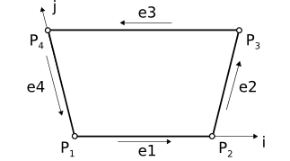


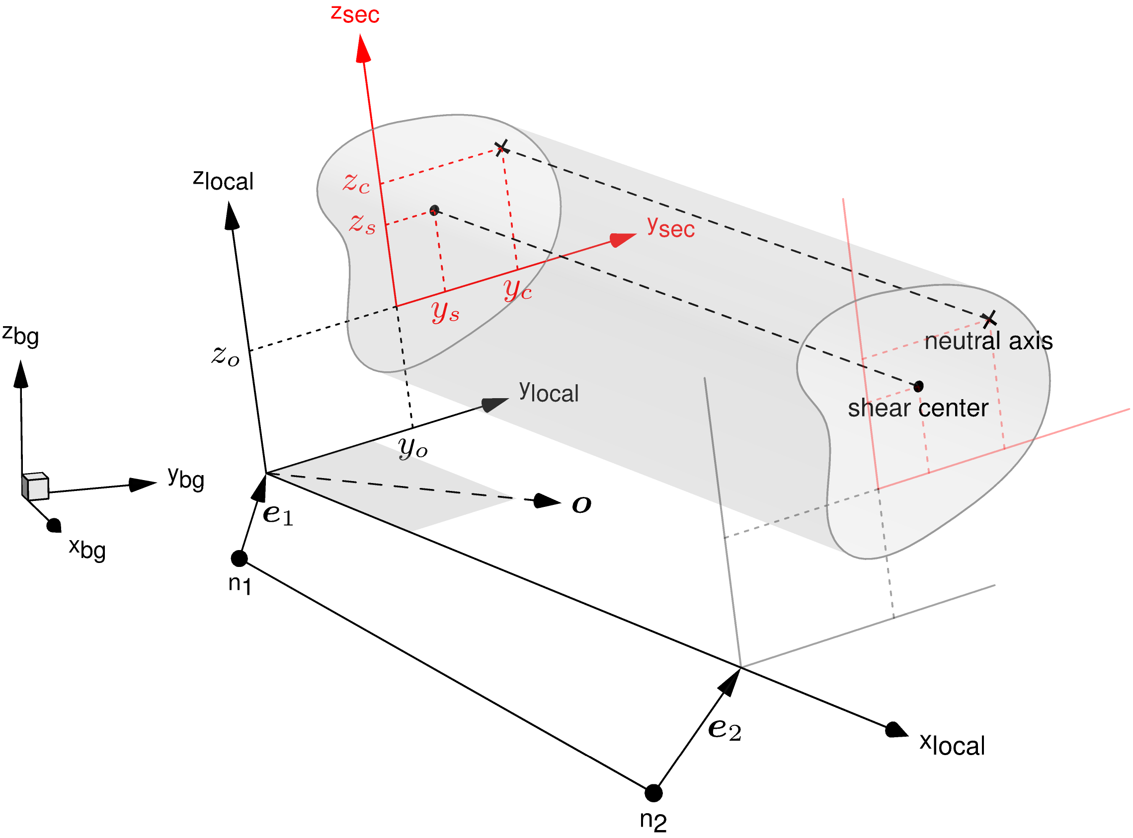


section origin
neutral axis
shear center
stress points (if any)