Introduction
b2000++ is a Finite Element problem solving environment made primarily to analyze the behavior of structures. With B2000++, you can predict with a high degree of accuracy the deformation field, the stress field, the buckling behavior, and the temperature distribution of many thin- and thick-walled, metallic and laminated composite structures. The modular architecture allows for extending its capabilities and to create plug-ins. b2000++ is operative under Linux and UNIX.
The b2000++ User Manual describes how to formulate a problem with b2000++'s Model Description Language and how to solve the problem with one of the b2000++ solvers.
Chapter Model Description Language (MDL) describes all ingredients of the MDL and how to combine them for formulation a FE model. The Model Description Language is a script-based data driven language for describing the geometrical, the physical, and the mathematical properties of a problem, and the numerical parameters for the solver(s).
Chapter Generic Elements describes the geometry and the element numbering of all b2000++ elements. The operator-specific elements are explained in the Chapter elements.
Chapter elements describes the MDL input parameters of all b2000++ operator-specific elements.
Chapter Solvers explains optional b2000++ solver parameters, specifically parameters to be included in the case block. The invocation of the solvers is explained in Chapter B2000++ Applications and the theoretical background can be found in the Section Solver Algorithms.
Additional information on solver algorithms, coordinate systems definitions, etc. can be found in the Chapter Selected Topics.
Chapter B2000++ Applications explains the invocation of the b2000++ applications. The theoretical background can be found in the Section Solver Algorithms.
Finally, the Selected Topics Chapter discusses specific subjects.
Work Flow
The work flow with B2000++ is a classical work flow for Finite Element analysis. An existing structure or a design of a structure to be studied must be modeled such that it fits in the scope and capabilities of a finite element analysis system. This modeling process includes decisions on the degree of approximation, both the continuum and the finite element model, the type of model to be created (beams, shell, solids). This process is not discussed here. The image below illustrates the work flow:

B2000++ analysis work flow
In the current version of B2000++ it is not planned to support the modification of the database with MDL commands. Modifications should be performed with Python scripts based on the MemCom Python module Python module.
An Example
A simply-supported thin quadratic laminated plate of 500 mm by 500 mm is loaded with a forced displacement along one of the plate edges. The linearized buckling load as well as the post-buckling response due to the forced displacement of the edge is to be determined.
The plate is simply supported on all four edges, one edge being free to move in the x-direction to allow for the forced displacement. The plate is loaded with a forced displacement loading condition along the free edge 2.

Geometry and loading of plate
The plate is made of a composite material, 16 layers of 0.125mm thickness, with the symmetric stacking sequence (in degrees) \((+45,0,-45,0,+4,0,-45,+90)_s\). The material data are listed below:
\(E_1 = 146.86\ 10^{3} N/mm^2\)
\(E_2 = E_3 = 9.65\ 10\ 10^{3} N/mm^2\)
\(\nu_232 = \nu_13 = 0.023\)
\(G_12 = G_23 = G_13 = 45.5\ 10^{2} N/mm^2\)
FE Model
Now we explain in detail how to get to the solution. We start by defining the Finite Element model with the B2000++ model description language (MDL). MDL contains simple mesh generation capabilities with element patches (epatch). A single epatch defines the regular plate mesh and links to the material.
(et="Q4.S.MITC.E4")
(ne=40)

# Mesh definition
epatch 1
  geometry plate  # Geometry type
  p1 0.   0.   0. # 4 plate vertices
  p2 500. 0.   0.
  p3 500. 500. 0.
  p4 0.   500. 0.
  eltype (et)     # Element type
  ne1 (ne)        # N. of elements in first direction
  ne2 (ne)        # N. of elements in second direction
  mid 2           # Link to material identifier
end
Note the parametrization of the element type and the number of elements. Here we select Q4 four node quadrilateral MITC elements.
The plate geometry is uniquely defined by the four corner points p1, p2, p3, and p4 specified counter-clockwise, supposing straight plate edges. Note that the plate thickness is not needed if the material is a laminate material.
A laminate is defined with the MDL material block, by listing all layers one after the other, each layer specifying the thickness, the layer orientation, and the material identifier.
# Composite stacking sequence definition
material 2
  type laminate
  0.125  45 1
  0.125   0 1
  ...
end
For our model the default global material orientation is selected, i.e the material angle is defined with respect to the global coordinate system as displayed in the figure above. See section B2000++ Materials.
The composite material constants are defined with
material block, specifying the orthotropic
material type.
material 1
  type orthotropic
  e1 146.86e+03
  e2 9.65e+03
  e3 9.65e+03
  nu12 0.3
  nu13 0.3
  nu23 0.023
  g1 45.5e+02
  g2 45.5e+02
  g3 45.5e+02
  failure max_principal_strain
    t +4500.e-6 # tension, micro-strain
    c -3000.e-6 # compression, micro-strain
    s +5000.e-6 # shear, micro-strain
    filter max_of_element
  end
end
A simple failure criterion is used, based on the maximum of the principal eigenvalues of the strain tensor. Its purpose is to select, for each element, the material point which is the most critical. This way, the amount of gradient data that is written to the database is reduced, which is important when working with laminate materials.
b2000++ discerns between essential boundary conditions (here: displacement constraints) and natural boundary conditions (here: forces). For our model we have to define the essential boundary conditions for (1) creating the required displacement constraints along edge 2 in the x-direction and (2) properly locking the structure along the edges.
Essential boundary conditions ebc along patch edges,
i.e displacement constraints, can be added by referencing the proper
epatch element (here: edge e2). MDL automatically generates the mesh
node and element lists. They are stored in the model database and can
be referenced by ebc and nbc boundary
condition definitions.
The first ebc block 1 locks the structure. Since the edges are free to rotate we only lock the displacement DOFs, i.e DOFs UX, UY, or UZ:
ebc 1
   # Zero-value constraints
   value  0. dof [  UY UZ] epatch 1 e1  epatch 1 e2  epatch 1 e3   epatch 1 e4
   value  0. dof [UX     ] epatch 1 e4
end
The first line of the ebc block locks the y- and
z-displacement DOFs of all edge nodes. The second line locks the
x-displacement DOFs of the edge opposite to the moving edge (e2).
The second ebc block 2 applies a value for the
x-displacement of all nodes of the edge e2:
ebc 2
   # Forced displacement
   value -1. dof  UX epatch 1 e2
end
The links to the ebc sets will be added to the case block, as will be described later.
For the particular configuration, i.e. a flat plate, an ‘imperfection’
has to be defined to trigger the post-buckling behavior. This can be
achieved by defining a small out-of-plane force that ‘pushes’ the
plate in the desired post-buckling direction (in the present model
only one configuration is possible). The out-of-plane concentrated
force of 1 N is assigned to the shell patch center node (identified
with the epatch node p9) with a nbc block:
# Central out-of-plane force to create imperfection
nbc
  set 1
    value 1. dof FZ epatch 1 p9
  end
end
Note that, if node-local coordinates systems are defined (this is typically the case for curved shells), boundary conditions are defined with respect to the local coordinate system of the nodes associated to the DOF. In this example, however, there are no node-local coordinate systems. Hence, all boundary conditions are expressed in the global coordinate system.
All parameters related to an analysis case description are contained in a case block. In out example we will carry out 2 types of analysis, a buckling analysis and a post-buckling analysis.
Buckling Analysis
The case block for the buckling analysis defines the type of analysis, includes the links to the boundary conditions, and, for the buckling analysis type, defines the number of buckling modes to be computed.
case 1
  analysis  linearised_prebuckling
  nmodes    10
  ebc       1
  ebc       2
  gradients 1
end

adir
  case 1
end
In the analysis case description above, the buckling solver is
activated for 10 buckling modes (note that selecting only a very small
number buckling modes, such as 1 or 2, might lead to numerical
problems in the eigensolver). The clamping and the displacement
boundary conditions (ebc 1 and ebc 2) are activated.
The buckling analysis is carried out by entering the shell command
b2000++ buckling.mdl
After the analysis has completed, the Simples script print_critical_loads.py
model = si.Model('buckling')
formatter = si.formatdb.BucklingLoad(model, case=1)
print(formatter.format())
prints the buckling factors and the buckling loads:
python  print_critical_loads.py
:emphasize-lines: 1

Total reaction force F=(-158593, -5.40012e-12, 4.22051e-15), amplitude Famp=158593

     Mode       Lambda   Crit. load
        1      0.01689         2678  *
        2      0.03735         5923  *
        3      0.04765         7557  *
        4      0.06436    1.021e+04  *
        5      0.07545    1.197e+04  *
        6      0.09728    1.543e+04  *
        7      0.09878    1.567e+04  *
        8       0.1177    1.866e+04  *
        9       0.1256    1.992e+04  *
       10        0.138    2.188e+04  *

Lambda (eigenvalue): if > 1 no buckling, < 1 buckling, marked by *
Critical load: F * Lambda (if F != 0)
Reaction force: Sum of reactions due to EBC and NBC
Results can also be viewed with the B2000++ browser. Enter the shell command below and click on “Solutions”, “case 1”, and “Buckling Loads”:
b2browser buckling
The buckling modes can be plotted with the baspl++ viewer. Enter the following shell command which displays the plate with the first buckling mode:
baspl++ plot_buckling_mode.py
The following image shows the shapes of some buckling modes:
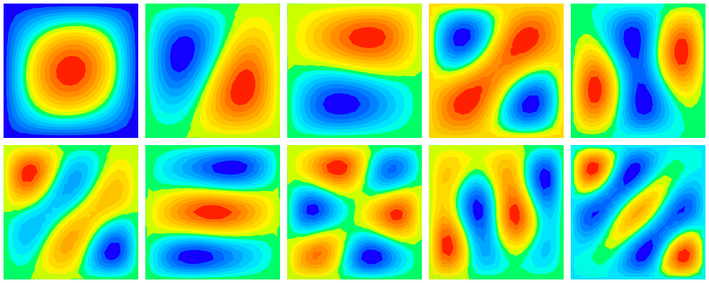
Buckling modes (amplitude plotted).
Post-Buckling Analysis
The case block for the post-buckling analysis defines the type of analysis, includes the links to the boundary conditions, and, for the buckling analysis type, defines the number of buckling modes to be computed.
case 1
   analysis        nonlinear
   ebc             1
   ebc             2 sfactor 0.1  # up to 0.1mm edge shortening
   nbc             1 sfunction 1. # constant force, not scaled by load factor
   step_size_init  0.01           # to get smoooth pre-buckling path
   step_size_max   0.01           # to get smoooth post-buckling path
   gradients       1              # compute gradients for all increments
   rcfo_restrict epatch 1 e2      # Restrict computation of reaction forces
                                  # to edge e2 nodes
end

adir
  case 1
end
The following comments pertain to the the post-buckling analysis case description above:
The
ebc 2link includes thesfactor 0.1, which means that the load is incremented up to 0.1 times theebc 2values.The
nbc 1link includessfunction 1.0, which means that the load ofnbc 1is applied constant during all increments.Setting
step_size_initandstep_size_maxboth to 0.01 , i.e. keeping the increments constant, will produce a smooth post-buckling path for the graphs, at the expense of higher computation time.2The
rcfo_restrictoption tells any post-processing tool, such as Simples, to restrict the computation of reaction forces to the nodes of the list (here: the epatch edge e2 nodes).The buckling analysis is carried out by entering the shell command
b2000++ postbuckling.mdl

INFO:solver.static_nonlinear:18:22:45.812: Start static nonlinear solver for case 1
INFO:solver:18:22:45.813: Resolving linear constraints: 102 equations.
INFO:solver:18:22:45.813: 0 dependent constraints were eliminated.
INFO:solver:18:22:45.813: Reduction matrix (903 x 1005) has 903 nonzeros.
INFO:solver.static_nonlinear:18:22:45.813: Start increment 1 of stage 1 for time 0 and time step 0.01.
INFO:solver.static_nonlinear:18:22:45.885: Start increment 2 of stage 1 for time 0.01 and time step 0.01.
...
INFO:solver.static_nonlinear:18:22:48.304: Start increment 99 of stage 1 for time 0.98 and time step 0.01.
INFO:solver.static_nonlinear:18:22:48.331: Start increment 100 of stage 1 for time 0.99 and time step 0.01.
INFO:solver.static_nonlinear:18:22:48.363: End static nonlinear analysis for case 1 with success.
After the analysis has completed, the Simples script plot_postbuckling_graphs.py
python plot_postbuckling_graphs.py
plots the graphs below:
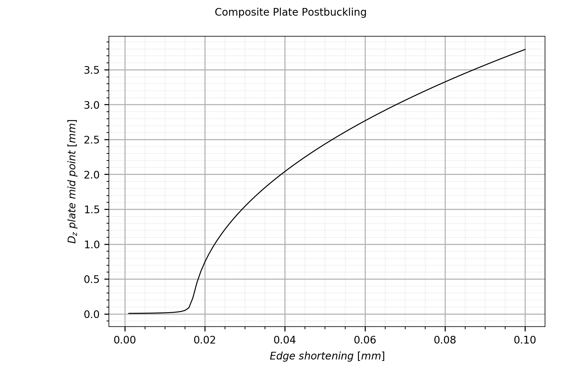
Mid-point out-of-plane displacement vs. edge shortening plot.
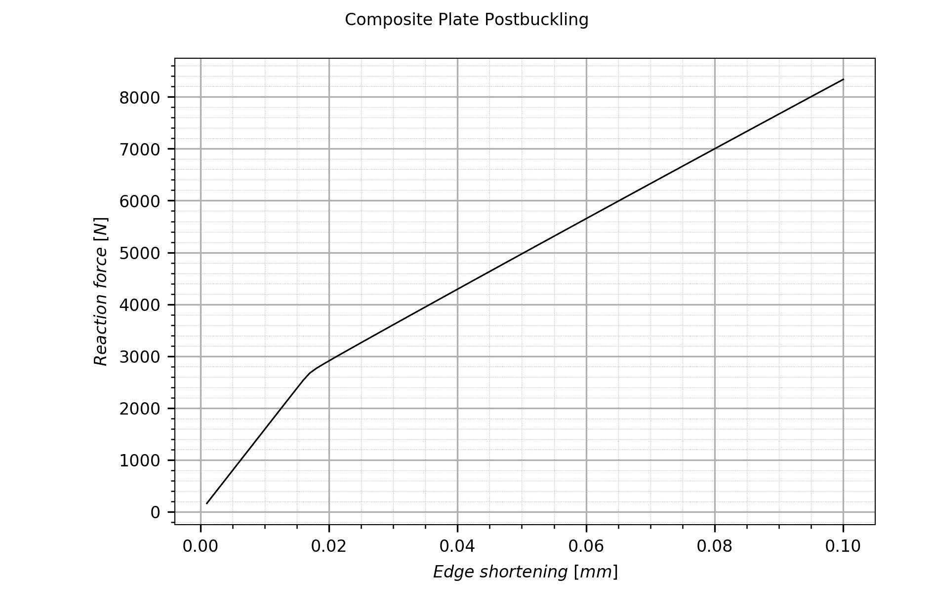
Total reaction force vs. edge shortening plot. The reaction force ist the sum of all reaction forces applied to epatch edge e3.
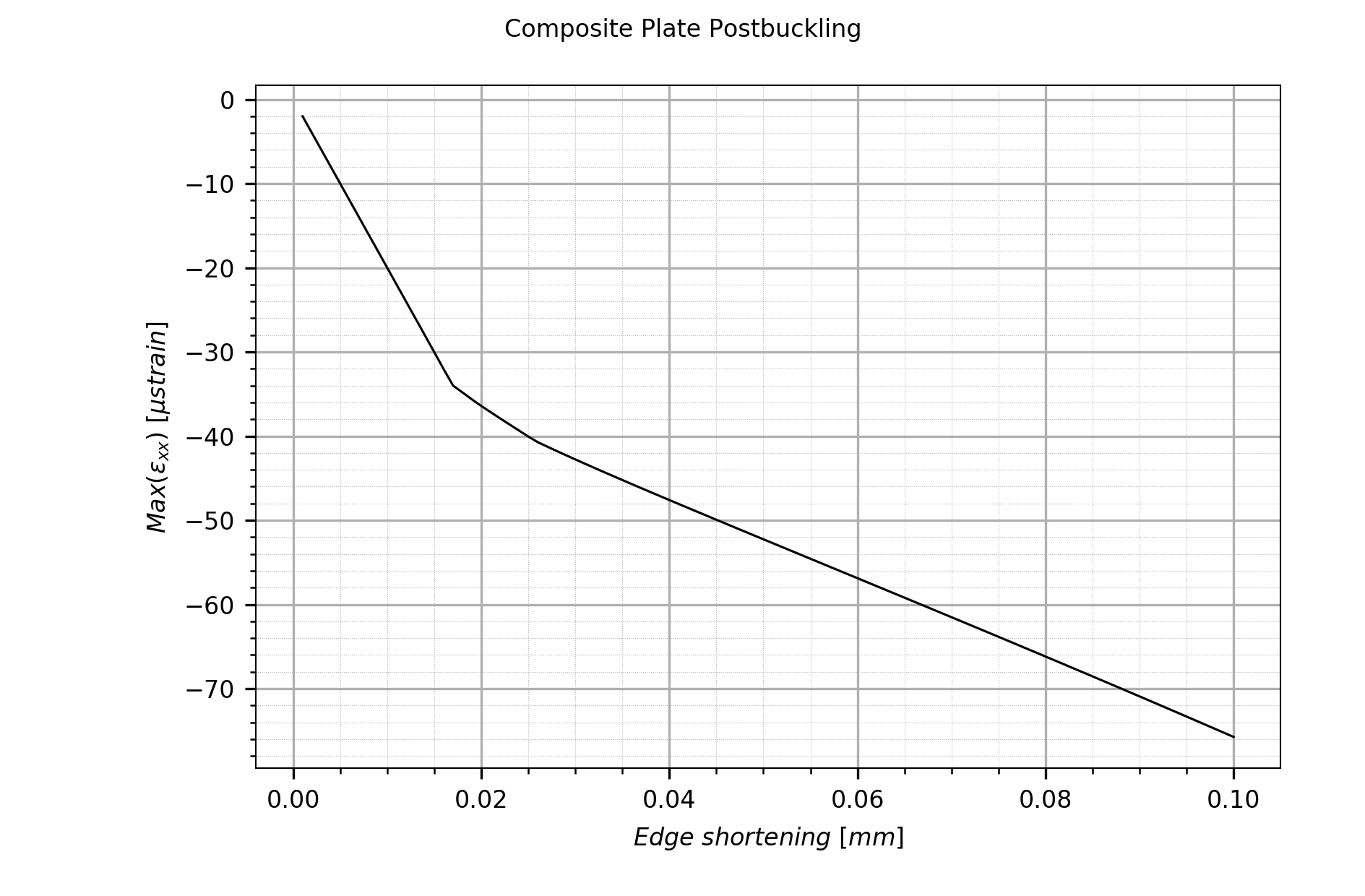
Maximum \(\epsilon_xx\) vs. edge shortening plot.