Linear static (stationary) or linearized problems are solved with the
linear static solver. It is activated for a specific case
with the analysis parameter linear.
If several load cases with the same constraints are present, the MDL subcase option can
be applied during linear analysis, reducing computation time (the
global matrix is the factored once and a back-substitution is
performed for each subcase).
Note
You cannot solve several cases with different analysis parameters in one solver run!
Nonlinear static (stationary) problems are solved with the nonlinear
static solver. It is activated for a specific case with the
analysis parameter nonlinear.
Note
You cannot solve several cases with different analysis parameters in one solver run!
A nonlinear problem is solved with an incremental procedure following
an increment control parameter denoted \(\lambda\).
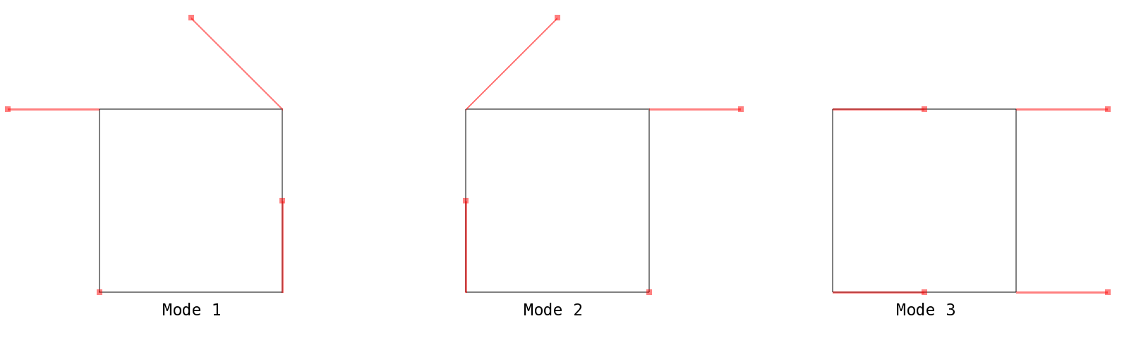
Five increment constraint strategies can by used with this solver. The
figure below illustrates these by a geometric representation for a
single DOF problem (DOF parameter plotted horizontally and control
parameter \(\lambda\) plotted vertically):
Geometric representation of constraint strategy for a single DOF
problem.
The correction strategy is of the Newton-iteration type, optionally
augmented with an acceleration method and a line search algorithm.
Optional Static Nonlinear Solver CASE Parameters
In addition to the MDL command analysisnonlinear, the following
commands may be specified in the case block.
correction_typenewton|accelerated_newton
Specifies the type of correction in a given Newton iteration. Default
is newton.
The newton correction type only makes use of the residuum and the
tangent matrix (updated or not) to compute the correction.
The accelerated_newton correction type is meaningful with a
modified Newton method. It monitors whether the sequence of Newton
iterations converges (whether the residuum decreases), and if not
(divergence), invokes the line search algorithm to find a better
solution. With line search, it is often possible to find a solution
outside the convergence region. Thus, when using the MDL commands
newton_methodmodified or newton_methoddelayed_modified,
the accelerated Newton correction can converge for larger time
steps than the normal Newton correction type.
Specifies the type of test which indicates whether the Newton
iterations of the correction phase have sufficiently converged. The
tests make use of some or all of the MDL commands tol_residuum,
tol_solution, and tol_work. Default is flux_normalised.
The flux_normalised correction termination test computes the
residuum normalised by the energy flux for each type of field
(displacements, rotations, Lagrange multipliers, etc.) separately.
The flux_normalised test has additional options, see
Flux-normalised Correction Termination Test.
The regularised correction termination test regularizes the
residuum, the solution changes, and the energy change, with the goal
of making the test independent of the units. Thus, changing the units
of an FE model (e.g. [kg,m,s]) to another (consistent) unit system
(e.g. [t,mm,s]) should not require modification of the tolerances.
The following tolerances are used: tol_residuum (default 1e-3),
tol_solution (default 1e-3), and tol_work (default 1e-7).
The dof_and_residue correction termination test tests the L2-norm
residuum against tol_residuum and the L2-norm of the solution
changes w.r.t. the previous Newton iteration against
tol_solution. The following tolerances are used: tol_residuum
(default 1e-3) and tol_solution (default 1e-3).
The normalised_dof_and_residue correction termination test
divides the L2-norm residuum by that of the first Newton iteration.
The same is done for the L2-norm of the solution changes w.r.t. the
previous Newton iteration. The following tolerances are used:
tol_residuum (default 1e-3) and tol_solution (default 1e-3).
gradientsVALUE
Controls the computation of the gradients (strains, stresses, heat
transfer, etc.) for the current case. If VALUE (int) is set to 0
(default) no gradients are computed and saved, i.e. only dof
solutions will be found on the database. If VALUE`issetto-1,thegradientsforthelastconvergedstepofatstageorthelinearsolutionsteparecomputedandsaved.If``VALUE is set to a positive
value, the gradients will be computed at each istep step of at
stage as well as for the last step of a stage.
gradients_onlyYES|NO
Specifies whether only gradients (and reaction forces) should be
computed, while the solution vector is defined solely by the the
initial conditions, and the boundary conditions and the current load
increment. Default is NO.
Specifies the increment constraint strategy to use. The increment
constraint strategy serves two purposes: It defines the increment
constraint for the predictor phase and the corrector phase, and it
computes the predictor solution from the solution of the last
converged step. This predictor solution is then used as initial
solution to the correction phase.
The following strategies are available: load means
load-controlled. To avoid singularities at limit points in
post-buckling analysis, residue_function_typeartificial_damping
can be used.
A state-controlled strategy is used with state.
The other strategies are of the continuation type. For the
hyperelliptic and local_hyperelliptic strategies, the
parameters hyperelliptic_a and hyperelliptic_b define the
size of the ellipse.
The initial step cycle number (int). Default is 1.
line_searchyes|no
Specifies whether line search should be used for the
accelerated_newton method (see the MDL command
correction_type). The line search method satisfies the strong
Wolfe condition. When the cost of calculating the first variation
is significantly lower than the cost of calculating the second
variation, it is recommended to have line search enabled, as it
improves the probability that the Newton iterations
converge. Default is yes.
max_divergencesVALUE
Defines the maximum number of consecutive divergences (int) during the
correction phase of a load step. Default is 4. When VALUE is
reached, the correction phase is terminated unsuccessfully, and the
step increment is re-started with a reduced step size.
max_newton_iterationsVALUE
Specifies the maximum number of Newton iterations (int) per
increment. Default is 50.
max_stepsVALUE
Maximum number of steps (increments) (int) per stage. Default
is 99999.
Specifies what kind of Newton method should be used. Default is
conventional.
The conventional method performs factorization for the
predictor and for each Newton iteration, and thus is a full Newton
method.
Forthemodified method, factorization of the tangent matrix is
performed when the correction phase has terminated unsuccessfully.
Hence, several increments may be performed without any
factorization.
The delayed_modified method performs a factorization for the
predictor and for the first Newton iteration.
Note that the artificial_damping option for the MDL command
residue_function_type enforces factorization each time the step
size changes. For the modified and delayed_modified Newton
methods, is is recommended to use the correction_typeaccelerated_newton option.
newton_periodic_updateVALUE
For the modified and delayed modified, non-accelerated Newton
methods, `` VALUE`` (int) specifies the maximum number of consecutive
iterations without re-factorization. When `` VALUE`` is reached, a
re-factorization will be performed, and the counter is reset. Note
that for high values of `` VALUE`` and depending on
the newton_method setting, several increments may be performed
until this number of Newton iterations is reached. Default is 100.
Specifies the type of residuum (first variation or internal forces
vector) and its derivative (second variation or tangent matrix).
The default type computes the first and second variation without
any modifications.
In a load-controlled post-buckling analysis involving collapse, the
artificial_damping type is necessary for the Newton iterations to
converge. It adds viscous forces to the residuum vector (first
variation). The velocities are computed from the difference of the
solution to the last converged solution, divided by the step size. To
the tangent matrix (second variation), the viscosity matrix divided
by the step size is added. With artificial damping, singularity of
the tangent stiffness matrix at limit points can be avoided and
energy can be dissipated during mode jumps. See also artificial
damping.
The scaled type scales the DOFs by their respective diagonal
element in the tangent matrix. This may be beneficial in continuation
analysis (e.g. increment_control_typelocal_hyperelliptic). Due
to the scaling, it is recommended to use the default correction
termination test.
step_size_initVALUE
Step size (float) at the beginning of the stage. Default is 0.1.
step_size_maxVALUE
Maximum step size (float) during the stage. Default is 1.0. In
continuation analysis, this is the size along the load path.
step_size_minVALUE
Minimum step size (float) during the stage. Default is 1e-12. In
continuation analysis, this is the size along the load path.
step_size_lambda_maxVALUE
Maximum lambda step size (float) during the stage in a continuation
method analysis. Default is 1.0.
step_size_lambda_minVALUE
Minimum lambda step size (float) during the stage in a continuation
method analysis. Default is 1e-12.
step_size_dof_maxVALUE
Maximum degrees of freedoms step size (float) during the stage in a
continuation method analysis. Default is 1.0.
step_size_dof_minVALUE
Minimum degrees of freedoms step size (float) during the stage in a
continuation method analysis. Default is 1e-12.
tol_residuumVALUE
The error tolerance value (float) for the residuum
(‘equilibrium’) error; used by the Newton correction termination
test. The default depends on the correction_termination_test
option.
tol_solutionVALUE
The error tolerance value for the dof (‘solution’) error; used by the
Newton correction termination test. The default value on the
correction_termination_test option.
tol_workVALUE
The error tolerance value (float) for the work error; used by some
Newton correction termination test. The default depends on the
correction_termination_test option.
The static solver is most commonly used for stress analysis involving
geometric, material, or boundary nonlinearity, and for heat transfer
analysis involving nonlinear material or boundary behavior.
Note
For load-controlled quasi-static stress analysis with artificial
damping, an alternative exists in the dynamic nonlinear
solver, which can also be used for
quasi-static stress analysis when specifying the MDL case parameters
Due to its predictor and its mechanism to control the time increment
by means of an error estimator, the dynamic nonlinear solver may be -
depending on the problem and depending on the solution parameters -
more effective than the static nonlinear solver.
The static solver can also steer a weakly-coupled multi-disciplinary
analysis, this is briefly explained for the case of steady-state
aero-elasticity: The spatial coupling, CFD mesh deformation, and CFD
solver are wrapped inside a specially-designed and implemented nonlinear
natural boundary condition object. For each Newton iteration, the static
solver evaluates the natural boundary condition for the solution field;
in this case, the boundary condition returns the spatially mapped
aerodynamic forces that were calculated from the deformed configuration.
Example: Load-Controlled Stress Analysis with Dissipation
In stress analysis, a problem may be considered highly nonlinear if
geometric instabilities, material nonlinearity such as degradation, or
contact conditions are present. A typical parameter specification for
such situations is:
Load control is enabled by default. For highly nonlinear problems, the
full Newton method (default) is often more expedient than the
accelerated modified Newton method. The default maximum number of
Newton iterations max_newton_iterations should be sufficient in
many cases. Lower values may cause many small time increments or even
failure to converge, while higher values may lead to increased
computation time. In case of very slow but reliable convergence,
higher values (100-200) may be necessary.
When using a load-controlled strategy, a mechanism to dissipate energy
must be enabled when instabilities occur. This is achieved with the
residue function type set to artificial_damping. The amount of
damping is controlled with the dissipated_energy_fraction
parameter. High values accelerate the analysis, increasing the
increment sizes, but may influence the results on the other
hand. Therefore, a compromise between analysis time and accuracy has
to be found. While the parameter value is independent of the physical
units, the necessary amount of damping depends on the problem. Thus,
the default of 1e-4 may not be appropriate. It is recommended to vary
this parameter in powers of 10 (e.g. make an analysis for 1e-7, 1e-6,
1e-5, 1e-4, 1e-3) and observe its effect.
When the problem is expected to be nonlinear from the start, an
initial step size may be specified with the step_size_init
option. The maximum step size should always be set, using the
step_size_max option, for the reason that different load paths may
be followed and collapse cannot be reliably predicted if the step size
is too large (the solver may “jump over” collapse paths). The default
of 1e-12 for the minimum step size is sufficient for most problems.
Another important option is max_divergences which may be used to
trigger collapse by using smaller values (1 or 2) than the default. On
the other hand, analyses involving material degradation may benefit
from higher values (increasing the chances that the Newton iterations
will converge).
Example: Post-Buckling Analysis
A typical static potentially highly nonlinear post-buckling analysis
parameter setting is
The parameter increment_control_typehyperplane enables a specific
method of continuation analysis, here the hyperplane method.
The maximum step size in thew loading-direction can be controlled by
means of the step_size_lambda_max option. Its counterpart is the
step_size_dof_max option which controls the maximum step size in
the DOF direction. The step_size_max option controls the
arc-length of the increments.
Example: Mildly Nonlinear Continuation Analysis
A typical static ‘mildly’ nonlinear post-buckling analysis
parameter setting is
The parameter increment_control_typehyperplane enables a specific
method of continuation analysis, here the hyperplane method. If
the problem is only mildly nonlinear (for instance, if no limit points
are expected), there is no need to limit the step size.
In this example, the delayed-modified Newton method is used in
conjunction with acceleration via line search.
The nonlinear analysis is attempted in a single increment, i.e. a
step_size_init of 1.0, which might not always work. In such cases,
the default of 0.1 is more expedient.
Load control is enabled by default. Due to the highly nonlinear
contact conditions, the full Newton method (default) is often more
expedient than the accelerated modified Newton method. Because the
Newton iterations may converge slowly when contact is active, a high
number of Newton iterations is allowed.
The maximum number of divergences is increased, this improves the
chances that the Newton iterations will converge.
If the contact conditions are enforced via quadratic penalties, the
tangent stiffness matrix may be, depending on the penalty factor,
badly conditioned. In this case, the tolerances for convergence may
need to be increased using the tol_residuum and tol_solution
options.
Nonlinear heat-transfer analysis is often well-behaved and therefore may
be carried out with the above settings.
Load-controlled analysis is enabled by default. Because the problem is
considered mildly nonlinear, there is no need to limit the step size,
and the delayed-modified Newton method (or the modified Newton method)
can used in conjunction with acceleration via line search.
Depending on the amount of detail required, the maximum step size may be
limited. Depending on the accuracy required, the tolerances for
convergence may be modified.
Linear dynamic (non-stationary) problems are solved with the linear
static solver. It is activated for a specific
case with the analysis parameter
`` dynamic_linear``.
Implicit time integration is performed in the linear dynamic linear
solver with the Newmark method and with a fixed time step size and
with one single stage.
Note
It is not recommended to solve dynamic problems with the dynamic
linear solver due to the above restrictions.
By default te time (load) step is 1. However the analysis duration is
usually not 1 (time unit), and an analysis stage must be defined in
the case definition, scaled by the duration. Refer to
the example below below
for details.
Optional Dynamic Linear Solver CASE Parameters
In addition to the MDL command analysisnonlinear, the following
commands may be specified in the case block.
gradientsVALUE
Controls the computation of the gradients (strains, stresses, heat
transfer, etc.) for the current case. If VALUE (int) is set to 0
(default) no gradients are computed and saved, i.e. only DOF
solutions will be found on the database. If VALUE is set to -1, the
gradients for the last converged step of at stage or the linear
solution step are computed and saved. Finally, if VALUE is set to a
positive value, the gradients will be computed at each istep step
of at stage as well as for the last step of a stage.
rayleigh_alpha|rayleigh_betaVALUE
Specifies the coefficients (float) for Rayleigh damping (default is 0). If
rayleigh_alpha and/or rayleigh_beta are set, Rayleigh damping
will be performed where the global viscosity matrix C is a linear
combination of the global mass and linear global stiffness matrices M
and K:
\[C = \alpha M + \beta K\]
step_sizeVALUE
Defines the step size (float) for the stage. No default is
given.
Example
A structure is fixed by means of an ebc (essential
boundary condition) while the dynamic load is applied by means of a
nbc (natural boundary condition), here a pressure
load. The Rayleigh damping coefficients have been calculated from a
free-vibration analysis. The analysis time is 10 s, and a step load is
applied during the first second.
The analysis time of 10 s is realized by having two cases, a case
(case 1) referencing a stage and a stage (stage 2) describing the
pulse. The step load is realized with the expression ‘t<1?1:0’, which
means that for t (the analysis time) between 0 and 1, the load is
applied with the factor 1, and for all the other time values the load
factor is 0.
Nonlinear dynamic (or non-stationary) problems are solved with the
dynamic nonlinear solver. It is activated for a specific
case with the analysis parameter
`` dynamic_nonlinear``.
Note
You cannot solve several cases with different analysis parameters in one solver run!
For the implicit time integration the dynamic nonlinear solver adopts
the backward differential formula (BDF) method which is well suited
for stiff ordinary differential equations [Sham79] like the ones
encountered in stress analysis. The second-order BDF is applied by
default, giving unconditional nonlinear stability. For computational
efficiency, the time step size is adapted during the analysis using
the Nordsieck transformation method [Nord62]. For stability and
accuracy of the time integration method, the rate of increment of the
step size is limited [Calvo87] and the step size is controlled using
Milne’s device error estimator [Milne70].
The solver is invoked by the MDL case parameter
analysisdynamic_nonlinear.
In general, the analysis duration is not 1 (second), and an analysis
stage must be defined in the case definition, scaled by
the duration. Refer to the first of the
examples below for details.
In stress analysis, the dynamic solver can be applied to problems
involving inertia forces or viscous forces. Like the static nonlinear
solver, the problem to be solved may involve any kind of geometric,
material, or boundary nonlinearities. Typical uses are:
Relaxation and creep analysis, in conjunction with visco-elastic
materials
Dynamic buckling analysis with or without artificial damping
Quasi-static buckling analysis with artificial damping
In heat-transfer analysis, typical applications are nonlinear loading
(e.g. cyclic loading) and predicting the non-stationary behavior (i.e.
the evolution of the temperature field). Like the static nonlinear
solver, the problem to be solved may involve any kind of material or
boundary nonlinearity.
Optional Dynamic Nonlinear Solver CASE Parameters
In addition to the MDL command analysisnonlinear, the following
commands may be specified in the case block.
Specifies the type of test which indicates whether the newton
iterations have sufficiently converged. Default is
flux_normalised.
The flux_normalised correction termination test computes the
residuum normalised by the energy flux for each type of field
(displacements, rotations, Lagrange multipliers, etc.) separately.
The flux_normalised test has additional options, see
Flux-normalised correction termination
test.
The dof_and_residue correction termination test tests the L2-norm
residuum against tol_residuum and the L2-norm of the solution
changes w.r.t. the previous Newton iteration against
tol_solution. The following tolerances are used: tol_residuum
(default 1e-3) and tol_solution (default 1e-3).
The normalised_dof_and_residue correction termination test
divides the L2-norm residuum by that of the first Newton iteration.
The same is done for the L2-norm of the solution changes w.r.t. the
previous Newton iteration. The following tolerances are used:
tol_residuum (default 1e-3) and tol_solution (default 1e-3).
gradientVALUE
Controls the computation of the gradients (strains, stresses, heat
transfer, etc.) for the current case. If `` VALUE`` (int) is set to
0 (default) no gradients are computed and saved, i.e. only DOF
solutions will be found on the database. If `` VALUE`` is set to
-1, the gradients for the last converged step of at stage or the
linear solution step are computed and saved. If `` VALUE`` is set
to a positive value, the gradients will be computed at each istep
step of at stage as well as for the last step of a stage.
line_searchYES|NO
Specifies whether line search should be used. Default is NO. This
line search method satisfies the strong Wolfe condition. When the
cost of calculating the first variation is significantly lower than
the cost of calculating the second variation, it is recommended to
activate line search, as it improves the probability that the Newton
iterations converge.
max_divergencesVALUE
Defines the maximum number of consecutive divergences (int) before
the step is reduced during a load step (optional). Divergence
occurs when the energy of the current correction is larger than the
energy of the preceding correction. Default is 4.
max_newton_iterationsVALUE
Maximum number of Newton iterations (int) per step. Default is 50.
max_stepsVALUE
Maximum number of steps or increments (int) per stage. Default is 99999.
multistep_integration_orderVALUE
Integration order (int) of the implicit transient integration
scheme. Currently supported values are 1 (Euler backward difference
formula), 2, 3, 4, 5, or 6. The solver is unconditionally
nonlinear-stable for values of 1 and 2. Default is 2.
Specifies what kind of Newton method should be used. Default is
conventional.
newton_periodic_updateVALUE
For the modified and delayed modified Newton methods, this option
specifies the maximum number of consecutive iterations (int)
without re-factorization. When this number is reached, a
re-factorization will be performed, and the counter is reset. Note
that for high values of newton_periodic_update and depending on
the newton_method setting, several increments may be performed
until this number of Newton iterations is reached. Default is 100.
Specifies the residue method (string). Default is order_n, for which the
MDL command multistep_integration_order defines the order of the
implicit time-integration.
The artificial_damping method works like in the static
nonlinear solver; the damping is of the Rayleigh viscous
type. Inertia effects are neglected, and the problem becomes a
first-order ODE. The global viscosity matrix is generated in
function either of the dissipated_energy_fraction option or the
rayleigh_alpha and rayleigh_beta options. In the first
case, the global viscosity matrix is a scaled instance of the mass
matrix, such that at the first increment, the ratio of the
dissipated energy to the total energy corresponds to the value
given in dissipated_energy_fraction. In the second case, the
global viscosity matrix is constructed in the same way as for
rayleigh_damping (see below).
For the rayleigh_damping (second-order) method, the global
viscosity matrix C is constructed from the global mass matrix M and
the global linear stiffness matrix K in the following way:
\[C = \alpha M + \beta K\]
The coefficient \(\alpha\) can be specified with the MDL
command rayleigh_alpha, and likewise, the coefficient
\(\beta\) can be specified with the MDL command
rayleigh_beta. Note that these coefficients can be determined
in the same way as explained in Artificial damping section for the static nonlinear
solver.
step_size_iniVALUE=v
Step size (float) at the beginning of the stage. Default is 0.1.
step_size_maxVALUE
Maximum step size (float) during the stage. Default is 1.0.
step_size_minVALUE
Minimum step size (float) during the stage. Default is 1e-12.
tol_dynamicVALUE
The dynamic nonlinear solver controls the step size with a local
error estimator, which is obtained with Milne’s method. VALUE`
(float) defines the maximum permitted absolute error of a degree of
freedom during one time step. Default is 1e-5. The step size is
adapted accordingly to this criteria. Setting VALUE to a large
value will inactivate the transient integration error control.
tol_residuumVALUE
Error tolerance value for the residuum (‘equilibrium’) error VALUE
(float) used by the Newton correction termination test. The default
depends on the correction_termination_test option.
tol_solutionVALUE
The error tolerance value for the dof (‘displacement’) error VALUE
(float) used by the Newton correction termination test. The default
depends on the correction_termination_test option.
tol_workVALUE
The error tolerance value for the work error VALUE (float) used by
the Newton correction termination test. The default depends on the
correction_termination_test option.
Example: Dynamic buckling stress analysis with Rayleigh damping
In this example, a panel is compressed in the x-direction by 3mm within
0.5s. If the analysis duration is different from the value of 1 (in time
units, usually seconds), a separate stage has to be defined, stage 2 in
the present example.
The duration of the analysis is given with the MDL command
stage2sfactorf
The amplitude of any specified boundary conditions in the stage must be
inversely-scaled by the analysis duration, this is done with the
sfactor option. On the other hand, the sizes for the minimum,
maximum, and initial step are given in absolute values. Hence,
step_size_init should always be defined.
The dynamic tolerance (tol_dynamic) option has a significant
influence on both accuracy and numerical effort. A large dynamic
tolerance leads to relatively large time step sizes, requiring many
Newton iterations per increment. Using a dynamic tolerance that yields
smaller time step sizes which require only one or two Newton iterations
is not only more accurate but often more effective. In some cases, a
modified Newton method may further reduce the computational effort.
Conversely, when the dynamic tolerance is set to an overly conservative
value, the resulting time step size may become extremely small in the
presence of high-frequency vibrations and fast movements.
When geometric instabilities are present, Rayleigh damping should be
selected (by setting the residue_function_type option to
rayleigh_damping and by setting the values for rayleigh_alpha
and rayleigh_beta) to ensure an effective solution process.
For highly nonlinear problems, the full Newton method (default) is often
more expedient than the modified Newton method. For mildly nonlinear
problems and for problems where the time step size is predominantly
limited by the time integration error, a modified Newton method may be
more effective. The default maximum number of Newton iterations
(50) should be sufficient in many cases. Lower values may
cause many small time increments or even failure to converge, while
higher values may lead to increased computation time. In case of very
slow but reliable convergence, higher values (100-200) may be necessary.
Example: Dynamic buckling stress analysis with visco-elastic materials
In this example, the options for Rayleigh damping are omitted since all
dissipation should come from the visco-elastic material. The dynamic
tolerance is crucial for the accuracy of the time integration: If the
time step sizes are too large, the numerical damping which is caused by
the time integration error may be larger than the material damping.
Example: Quasi-static buckling stress analysis with artificial damping
The dynamic solver can also be applied to load-controlled quasi-static
analysis. In this case, the analysis duration is irrelevant, and a
separate stage does not need to be defined. Also in this case, the
dynamic tolerance controls the time step size and is important to
computational efficiency and accuracy.
Energy is dissipated with artificial damping; the
residue_function_typeartificial_damping option also tells the
solver to neglect inertia forces. The amount of damping is controlled
with the dissipated_energy_fraction parameter. High values
accelerate the analysis, increasing the increment sizes, but may
influence the results on the other hand. Therefore, a compromise between
analysis time and accuracy has to be found. While the parameter value is
independent of the physical units, the necessary amount of damping
depends on the problem. Thus, the default of 1e-4 may not be
appropriate. It is recommended to vary this parameter in powers of 10
(e.g. make an analysis for 1e-7, 1e-6, 1e-5, 1e-4, 1e-3) and observe its
effect.
Example: Mildly nonlinear heat-transfer analysis
An initial temperature field is given (dof_init), and a constant
temperature is applied at the boundary (ebc1sfunction'1'). If
the problem is well behaved, it can be solved with a higher-order BDF
that is more accurate but not unconditionally stable, and a modified
Newton method can be used.
The analysis duration is one year (365 days), and the time step size
is fixed to one day (84600 seconds). A very large dynamic tolerance is
used to inactivate the solver’s error estimator.
Free vibration problems are solved with the frequency-independent free
vibration analysis solver. It is activated for a specific
case with the analysis parameter
`` free_vibration``.
Note
You cannot solve several cases with different analysis parameters in one solver run!
When executing b2000++ errors of the following kind
may indicate that the number of eigenmnodes nmodes to be
computed option should be increased.
Optional Free Vibration Solver CASE Parameters
In addition to the MDL command analysisnonlinear, the following
commands may be specified in the case block.
m_orthonormalyes|no
By default the mode shapes are normalized with respect to the mass
(“M-orthonormalized”), see [Bathe96]. If mode shapes should be
normalized to the maximum component of each mode (infinity norm),
set m_orthonormal to no.
nmodesVALUE
Number of free-vibration modes VALUE (int) to be computed. Must be
greater or equal to 2. It is often necessary to set this option to
values of 10 or even 20 for the successful solution of the
eigenvalue problem. Default is 2.
shiftVALUE
The spectral frequency (not the circular frequency!) shift value
VALUE (float). The computed free-vibration modes are the ones whose
eigen-frequency is near this value. For complex problems, a complex
spectral frequency shift value can be provided. Default is 0.
which_eigenvalues=sm|la|ra
Indicates where to search for eigenvalues with respect to 0 or to
the current shift value. sm searches for the smallest
eigenvalues around 0 or the current shift value (default). la
searches for the smallest eigenvalues to the left of 0 or the
current shift value. ra searches for the smallest eigenvalues
to the right of 0 or the current shift value.
matrices_dirVALUE
If set to a non-empty string, the free vibration solver will output the
system matrices as CSV formatted files in the directory provided by the
string VALUE.
The directory is created if it does not exist yet and populated by
the respective system matrices.
The provided path may be absolute or relative, relative directories are
created in the working directory of the solver.
By default an empty string is used, which deactivates the output.
To activate the output but write the files directly into the working
directory, provide a string like "./" for this option.
The frequency-dependent undamped vibration solver allows for solving
frequency-dependent free vibration eigenvalue problems to determine
eigenfrequencies and eigenmodes, where the linear internal forces and
internal inertia are frequency-dependent. It is activated for a
specific case with the analysis
parameter frequency_dependent_free_vibration.
Note
You cannot solve several cases with different analysis parameters in one solver run!
When executing b2000++, errors of the following kind
are indicative that the value for the nmodes option should be
increased.
Optional Frequency-Dependent Free Vibration Solver CASE MDL Parameters
In addition to the MDL command analysisfrequency_dependent_free_vibration, the following commands may be
specified in the case block.
nmodesVALUE
Number of free-vibration modes VALUE (int) to be computed (default:
1). It is often necessary to set this option to values of 10 or
even 20 for the successful solution of the eigenvalue problem.
shiftVALUE
The spectral frequency shift value VALUE (float). The computed
free-vibration modes are the ones whose eigenfrequencies are near
this value (default=0). For complex problems, a complex spectral
frequency shift value can be provided.
freq_initVALUE
The initial frequency VALUE (float) used in the first stage of the
algorithm.
tolVALUE
The relative tolerance VALUE (float) of the computation of the
exact eigenfrequency.
tol_predictorVALUE
The relative tolerance VALUE (float) for the re-computation of the
approximated eigenfrequencies.
The linearized pre-buckling solver is commonly used in stress analysis
of slender or thin-walled structures. It allows for the direct solving
of ‘buckling’ problems around an equilibrium position along the
nonlinear path. The linearized pre-buckling solver is activated for a
specific case with the analysis
parameter linearised_prebuckling.
Note
When executing b2000++, warnings of the following kind
are indicative that the value for the nmodes option should be
increased.
Optional Linearized Pre-Buckling Solver CASE Parameters
nmodesVALUE
Number of buckling modes v to be computed (default: 1). It is often
necessary to set this option to values of 10 or even 20 for the
successful solution of the eigenvalue problem.
shiftVALUE
The spectral frequency shift value. The computed buckling modes are
the ones whose eigenvalues (load factors) are near this value. The
default of 0 selects the nmodes lowest buckling modes.
In linear and nonlinear FE analysis, symmetric/unsymmetrc/real/complex
linear equation systems must be solved. In most cases, the matrices are sparse,
and often, they are symmetric as well. The solution of these systems of
linear equations constitutes an important part of the FE solving
procedures and as such has a great influence on the robustness and
effectiveness of any FE analysis. b2000++ automatically detects whether the
problem is symmetric/unsymmetrc/real/complex.
b2000++ offers several sparse linear equation solvers. By default, the
specific FE solvers (linear, nonlinear, static, dynamic)
automatically select the proper sparse linear equation solver. This
selection can be inactivated by forcing a specific sparse linear
equation solver by means of the case parameter
sparse_linear_solver. The following sparse linear equation solvers
are available in the current version of b2000++:
The MUMPS sparse linear equation solver is a direct multi-frontal solver for
use with general symmetric matrices. DMUMPS is the
default b2000++ sparse linear equation solver. It is particularly robust and effective on matrices
with Lagrange multipliers (i.e whenever nonlinear constraints
are present in the FE model). The parallel version is activated via the
mpirun command.
DMUMPS optional CASE Parameters
autospc=yes|no
Enables elimination of singular or nearly-singular degrees-of-freedom
(DMUMPS/DMUMPS_DP solvers only!). Default is
no. This option may be useful for example in conjunction with
Lagrange multipliers, or shell elements with free 6th
degrees-of-freedom.
The autospc option should be used with caution as it may significantly
influence the solution in non-foreseeable ways, especially in free-vibration
analysis and in linearized buckling analysis. For shell FE models, it is
recommended to use artificial drill stiffness instead.
autospc_valueVALUE
If autospc is enabled, use VALUE (float) to fix singular or
nearly-singular degrees-of-freedom DMUMPS/DMUMPS_DP
solvers only!). A value of 0.0 indicates that the autospc value
should be determined automatically. Default is 0.0. MUMPS
CNTL(4)=VALUE i.e CNTL(4) “determines the threshold for static
pivoting” (MUMPS documentation).
autospc_thresholdVALUE
If autospc is enabled, use VALUE (float) to determine
singular or nearly-singular degrees-of-freedom
(DMUMPS/DMUMPS_DP solvers only!). A value of 0.0
indicates that the autospc threshold will be chosen automatically.
Default is 0.0. MUMPS CNTL(2)=VALUE i.e CNTL(2) is “stopping
criterion for iterative refinement” (MUMPS documentation).
compute_null_space_vector=n
If autospc is enabled, compute a maximum of n (int) first null space
vectors (zero-energy modes) and store them on the database as DISP_NS
datasets(not documented). Default is 0.
Use of this option may require to adjust autospc_threshold.
The following example is a single 2D quadrilateral element. No
degrees-of-freedom are constrained, hence 3 zero-energy modes
are present.
When the MUMPS out-of-core solver is active, d (string) ist the
directory path name where the temporary files should be
created. By default, the /tmp directory is used.
mumps_ooc_prefix=d
When the MUMPS out-of-core solver is active, specifies d
(string) as prefix for the temporary files.
mumps_icntlVALUE
Sets one or several values in the MUMPS solver ICNTL (int) array, which is
used to control the behavior of the MUMPS solver. The string
VALUE consists of comma-separated key:value pairs, where
key is the index into the ICNTL array, starting from 1,
and value is an integer number.
The following example enforces the use of the
SCOTCH library for pivoting by
setting “ICNTL(7)=3”:
To also use iterative refinement with a fixed number of 3
iterations use:
mumps_icntl"7:3,10:-3"
In rare cases it is necessary to set ICNTL, the defaults
that are set by b2000++ are usually satisfactory or are
supported directly. While ICNTL allows to fine-tune the
workings of MUMPS, not all options will work with b2000++, and
the options 5 (matrix format) and 18
(matrix distribution) are forbidden, as they are determined
by b2000++ itself.
Refer to the MUMPS user’s guide, section 5.1, for an
explanation of ICNTL.
mumps_cntlVALUE
Sets one or several values in the CNTL (floating-point) array,
which is used to control the behavior of the MUMPS solver. The
string VALUE consists of comma-separated key:value pairs,
where key is the index into the CNTL array, starting from
1, and value is a floating-point number.
Only in rare cases it is required to set CNTL, the defaults
that are set by b2000++ are usually satisfactory or are
supported directly (e.g. autospc_threshold and
autospc_value).
One setting that may be of particular interest is CNTL(3),
which controls the threshold for identifying null pivots.
Since MUMPS 5.4.0 the criterion for the default setting CNTL(3)=0
defines a threshold relative to the sup norm of the preprocessed
matrix based on the machine precision and a factor dependent on the
number of variables on the deepest elimination branch. When provided a
positive value, this one is used instead of the machine precision and
factor for the calculation and a negative value is used directly as
an absolute threshold.
If the simulation aborts due to a null pivot it may help to set
the threshold to a value smaller than machine precision.
As it is possible to correctly represent 18 decimal digits in the
80 bit extended precision of x86 processors, we suggest to try
mumps_cntl"3:1.e-18" as a starting point if the default
threshold does not work.
Note: In older versions of MUMPS (before 5.4.0) the default value was
a factor of 1.e-5 below machine precision. To emulate that behaviour
set mumps_cntl"3:1.1e-21"
Refer to the MUMPS user’s guide, section 5.2, for an explanation
of CNTL.
Parallel direct left-looking super-nodal solver with static
pivoting, for use with positive-definite symmetric matrices,
making use of the the PASTIX library. Works obly if library is installed
In b2000++, the solver is executed with multi-threading enabled
and MPI and out-of-core support disabled.
Constraints originate from prescribed conditions such as
ebc, linc, field_transfer or
rigid-coupling (RBE elements) or distributed-coupling (FMDE) elements.
b2000++ supports different ways for imposing constraints on a FE
problem. Constraints may be linear or nonlinear, and may be imposed by
boundary conditions and by Finite Elements. For many problems, the
default settings (reduction for linear constraints and Augmented
Lagrange method or Lagrange method for nonlinear constraints) will
suffice to effectively obtain a solution. In this chapter, the MDL
commands for overriding these settings are described.
Optional Solver MDL Parameters
The following commands may be specified in the case
block.
Selects the type of method used to impose linear constraints on the
equations.
reduction
The system of linear equations is modified such that the
constraints are eliminated. The constraints are satisfied
‘exactly’ (within numerical precision). This is the default
method, and it is applicable to linear and nonlinear problems, but
only for linear constraints.
augmented_lagrange
A combination of Lagrange multipliers and penalties is used to
enforce the constraints. The MDL command
constraint_penalty specifies the penalty factor (default
value 1, it is rarely necessary to change this value). The
penalty factor is solely used to ensure the
positive-definiteness of the matrix and does not impair the
matrix’ condition number. The constraints are, due to the
Lagrange multipliers, satisfied ‘exactly’ (within numerical
precision).
Linear systems containing Lagrange multipliers are best solved
using a pivoting solver. It is recommended to use
sparse_linear_solver=dmumps, which is the default.
penalty
With the penalty method, the number of degrees-of-freedom remains
unchanged. The constraints are imposed approximately, where the
MDL command constraint_penalty specifies the penalty factor (default
value is 1e10). A high penalty factor ensures a close
approximation of the constraints but makes the matrix badly
conditioned; while a low penalty factor may introduce artifacts in
the solution of the FE analysis, especially for eigenmode
problems.
lagrange
To the system of linear equations, Lagrange multiplicators are
added. The constraints are satisfied ‘exactly’ (within numerical
precision).
Linear systems containing Lagrange multipliers are best solved
using a pivoting solver. It is recommended to use
sparse_linear_solverdmumps, which is the default.
Selects the type of method used to impose nonlinear (linearized)
constraints on the equations.
augmented_lagrange
A combination of Lagrange multipliers and penalties is used to
enforce the constraints. The MDL adir command
constraint_penalty specifies the penalty factor (default
value 1, it is rarely necessary to change this value). The
penalty factor is solely used to ensure the
positive-definiteness of the matrix and does not impair the
matrix’ condition number. The constraints are, due to the
Lagrange multipliers, satisfied exactly.
Linear systems containing Lagrange multipliers are best solved
using a pivoting solver. It is recommended to use
sparse_linear_solverdmumps, which is the default.
penalty
With the penalty method, the number of degrees-of-freeom
remains unchanged. The constraints are imposed approximately,
where the MDL adir command constraint_penalty
specifies the penalty factor (default value is 1e10). A high
penalty factor ensures a close approximation of the constraints
but makes the matrix badly conditioned; while a low penalty
factor may introduce artefacts in the solution of the FE
analysis, especially for eigenmode problems.
lagrange
To the system of linear equations, Lagrange multiplicators are
added. The constraints are satisfied exactly. Since for the static
case, the matrix is no longer positive definite, an unsymmetric
solver should be used.
Linear systems containing Lagrange multipliers are best solved
using a pivoting solver. It is recommended to use
sparse_linear_solver=dmumps, which is the default.
This is the default test to determine convergence of the Newton
iterations. The flux can be considered a measure of the individual
internal and external forces in the FE model. For each Newton
iteration, the instantaneous flux is normalised by the average
flux. The average flux is computed from the converged solutions of the
previous steps and from the solution of the current Newton iteration.
For all fluxes, and for the Newton correction of the solution, the
inf-norm (maximum) is used.
The flux normalization is performed per field, because each field may
have a different unit and a different range of values. The finite
elements present in the analysis model define what fields are active.
The following fields are commonly used in elastic analysis and
heat-transfer analysis:
Field name
Description
DISPLACEMENT
The displacement
degrees-of-freedom.
ROTATION
The rotational degrees-of-freedom
in shell and beam elements and in
rigid-coupling elements.
LAGRANGE
The degrees-of-freedom associated
to Lagrange multipliers.
TEMPERATURE
The degrees-of-freedom in
heat-transfer elements.
The following case parameters are active for all fields:
max_newton_iterationsVALUE
Specifies the maximum number of Newton iterations VALUE (int) per
increment. Default is 50.
max_divergencesVALUE
Defines the maximum number of consecutive divergences VALUE (int)
during the correction phase of a load step. Default is 4. When this
number is reached, the correction phase is terminated
unsuccessfully, and the step increment is re-started with a reduced
step size.
min_newton_iterations_check_divergenceVALUE
Checks divergence only after VALUE (int) Newton iterations. Default
is 4.
The following options can be specified either for all fields or per
field. In the second case, the field name must be appended to the relevant case parameter. Example:
case1ebc1analysis=nonlineartol_residuum=1.e-3# for all fieldstol_residuum.rotation=1.e-5# only for the rotation fieldend
tol_residuumv
Threshold for convergence: The maximum flux divided by the average
flux must be smaller than VALUE. Default is 1e-5.
tol_solutionv
Threshold for convergence: The maximum of the Newton correction,
divided by the maximum of the current step increment must be smaller
than VALUE. Default is 1e-5.
tol_residuum_linear_problemv
Threshold for linear convergence: If the maximum flux divided by the
average flux is smaller than VALUE, linear convergence is assumed,
without consideration of tol_solution. Default is 1e-8.
nb_iter_nonquadratic_convergencev
Number of Newton iterations that will be executed until the
convergence history will be examined to determine whether quadratic
convergence has been obtained. Default is 9 iterations.
tol_residuum_nonquadratic_convergencev
If convergence is not quadratic, after
nb_iter_nonquadratic_convergence Newton iterations,
tol_residuum is replaced by VALUE. Default is 2e-2.
average_fluxv
Use VALUE to normalise the flux, instead of the averaged flux which
is computed from the analysis.
initial_average_fluxv
Use VALUE as start value to compute the averaged flux. Default is
0.01.
zero_flux_criterionv
If the magnitude of the instantaneous flux divided by the averaged
flux is smaller then VALUE, the flux will be considered zero, and
tol_solution_zero_flux will be used instead of tol_solution.
Default is 1e-5.
tol_solution_zero_fluxv
Replaces tol_solution for fields having zero flux. Default is
1e-5.
zero_flux_relative_criterionv
For the computation of the normalised flux, discard regions in the
model where the flux is below VALUE. Default 1e-5.