Selected Topics

Analysis Cases

The Analysis Cases case refer to the ingredients to be used for an analysis. Specifically, they enumerate the boundary condition sets and other constraint sets as well as any additional sets required for a specific analysis. In addition, the analysis type and the corresponding analysis parameters, as well as numerical parameters, may be specified (these will override the analysis type and parameters defined in the adir analysis directives).

The case mechanism work as follows: The keyword cases of the ADIR dataset contains the list of case identifiers to be processed or solved for. This list is subset of the defined cases.

Each case is defined by the MDL case command and described on the database under the identifier CASE.id, where id is a positive integer.

Example of a case definition

A case with identifier 7 is defined by

• A reference to an essential boundary condition set 3.

• A reference to 2 natural boundary condition sets 15 and 7

• A reference to a linear constraint set

• A reference to a branch connectivity set.

The solver will then produce (1) the constraint set for case 7 with the EBC dataset set, the linear constraint set LINC dataset, and the JCTS dataset branch connectivity set and (2) the right hand side (natural boundary condition) with the sum of the NBC dataset sets 15 and 7.

Case definition example.

Solver Algorithms

Linear Static Solver Numerical Algorithm

The static linear problem exposed by the model abstraction layer of B2000++ is:

\[\begin{split}\left\{ \begin{array}{l} {F_{int}u + f_{int} = F_{ext}u + f_{ext}} \\ {u = {Rv} + r} \\ {Lu + l = 0} \\ \end{array} \right.\end{split}\]

where \(F_{int}u + f_{int}\) is the linearized internal value of the domain (the internal force in a displacement based formulation), \(F_{ext}u + f_{ext}\) is the linearized natural boundary condition (the external force in a displacement based formulation), \(R\) and \(r\) is the linearized model reduction, \(L\) and \(l\) is the linearized essential boundary condition.

Using the model reduction equation, the problem becomes:

\[\begin{split}\left\{ \begin{array}{l} {R^{T}\left( F_{int} - F_{ext} \right)Rv = R^{T}\left( f_{ext} - f_{int} \right) + R^{T}\left( F_{ext} - F_{int} \right)r} \\ {LRv = - Lr - l} \\ \end{array} \right.\end{split}\]

Using the Lagrange Multiplier Adjunction method for imposing the essential boundary conditions, the problem becomes:

\[\begin{split}\begin{bmatrix} {R^{T}\left( F_{int} - F_{ext} \right)R} & {R^{T}L^{T}} \\ {LR} & 0 \\ \end{bmatrix}\begin{bmatrix} v \\ \Lambda \\ \end{bmatrix} = \begin{bmatrix} {R^{T}{\left( f_{ext} - f_{int} \right) + R^{T}\left( F_{ext} - F_{int} \right)r}} \\ {- Lr - l} \\ \end{bmatrix}\end{split}\]

This linear system is solved and the solution \(u\) is then obtained form the linearized model reduction equation.

The difference of the natural boundary condition with the internal value of the domain (this is the reaction force in a displacement based formulation) is then:

\[f_{reac} = {\left( F_{int}u + f_{int} \right) - \left( F_{ext}u + f_{ext} \right)}\]

Nonlinear Solver Numerical Algorithm

A incremental-iterative algorithm, also called predictor-corrector method, is used to solve this problem. A stage is broken down into increments and for each increment a corrector phase is applied.

The static nonlinear problem exposed by the model abstraction layer of B2000++ is:

\[\begin{split}\left\{ \begin{array}{l} {f_{int}\left( {u,\lambda} \right) = f_{ext}\left( {u,\lambda} \right)} \\ {u = g\left( v,\lambda \right)} \\ {h\left( u,\lambda \right) = 0} \\ \end{array} \right.\end{split}\]

After imposing the reduction, the problem becomes:

\[f_{int}\left( {{g\left( {v,\lambda} \right)},\lambda} \right) = f_{ext}\left( {{g\left( {v,\lambda} \right)},\lambda} \right)\]

\[h\left( {{g\left( {v,\lambda} \right)},\lambda} \right) = 0\]

The potential energy of the unconstrained problem noted \(\Pi\left( {u,\lambda} \right)\) is defined by this first-order variation.

\[\nabla_{u}\Pi\left( {u,\lambda} \right) = f_{int}\left( {u,\lambda} \right) - f_{ext}\left( {u,\lambda} \right)\]

Thus we have:

\[\nabla_{v}\Pi\left( {v,\lambda} \right) = \nabla_{v}^{T}g\left( {v,\lambda} \right)\left( {f_{int}\left( {{g\left( {v,\lambda} \right)},\lambda} \right) - f_{ext}\left( {{g\left( {v,\lambda} \right)},\lambda} \right)} \right)\]

To impose the constraint, define Lagrange multipliers \(\Lambda\) to form the Lagrangian:

\[\mathcal{L}\left( {v,\Lambda,\lambda} \right) = \Pi\left( {v,\lambda} \right) + \Lambda^{T}h\left( {{g\left( {v,\lambda} \right)},\lambda} \right)\]

The first-order derivatives are:

\[\nabla_{v}\mathcal{L}\left( {v,\Lambda,\lambda} \right) = \nabla_{v}^{T}g\left( {v,\lambda} \right)\left( {f_{int}\left( {{g\left( {v,\lambda} \right)},\lambda} \right) - f_{ext}\left( {{g\left( {v,\lambda} \right)},\lambda} \right) + \nabla_{u}^{T}h\left( {{g\left( {v,\lambda} \right)},\lambda} \right)\Lambda} \right)\]

\[\nabla_{\Lambda}\mathcal{L}\left( {v,\Lambda,\lambda} \right) = h\left( {{g\left( {v,\lambda} \right)},\lambda} \right)\]

\[\nabla_{\lambda}\mathcal{L}\left( {v,\Lambda,\lambda} \right) = c\left( {v,\Lambda,\lambda} \right)\]

where \(c\left( v,\Lambda,\lambda \right)\) is the increment constraint condition that defines the increment control strategy.

The second-order derivatives are:

\[\nabla_{vv}\mathcal{L}\left( {v,\Lambda,\lambda} \right) = \nabla_{v}^{T}g\left( {v,\lambda} \right)\left( {\nabla_{u}f_{int}\left( {{g\left( {v,\lambda} \right)},\lambda} \right) - \nabla_{u}f_{ext}\left( {{g\left( {v,\lambda} \right)},\lambda} \right)} \right)\nabla_{v}g\left( {v,\lambda} \right) + \nabla_{vv}^{T}g\left( {v,\lambda} \right)\left( {\nabla_{u}f_{int}\left( {{g\left( {v,\lambda} \right)},\lambda} \right) - \nabla_{u}f_{ext}\left( {{g\left( {v,\lambda} \right)},\lambda} \right)} \right) + \nabla_{vv}^{T}h\left( {{g\left( {v,\lambda} \right)},\lambda} \right)\Lambda\]

\[\nabla_{v\Lambda}\mathcal{L}\left( {v,\Lambda,\lambda} \right) = \nabla_{v}^{T}g\left( {v,\lambda} \right)\nabla_{u}^{T}h\left( {{g\left( {v,\lambda} \right)},\lambda} \right)\]

\[\nabla_{v\lambda}\mathcal{L}\left( {v,\Lambda,\lambda} \right) = \nabla_{v}^{T}g\left( {v,\lambda} \right)\left( {\left( {\nabla_{u}f_{int}\left( {{g\left( {v,\lambda} \right)},\lambda} \right) - \nabla_{u}f_{ext}\left( {{g\left( {v,\lambda} \right)},\lambda} \right)} \right)\nabla_{\lambda}g\left( {v,\lambda} \right) + \nabla_{\lambda}f_{int}\left( {{g\left( {v,\lambda} \right)},\lambda} \right) - \nabla_{\lambda}f_{ext}\left( {{g\left( {v,\lambda} \right)},\lambda} \right)} \right) + \nabla_{v\lambda}^{T}g\left( {v,\lambda} \right)\left( {f_{int}\left( {{g\left( {v,\lambda} \right)},\lambda} \right) - f_{ext}\left( {{g\left( {v,\lambda} \right)},\lambda} \right)} \right) + \nabla_{u\lambda}^{T}h\left( {{g\left( {v,\lambda} \right)},\lambda} \right)\Lambda\]

\[\nabla_{\Lambda v}\mathcal{L}\left( {v,\Lambda,\lambda} \right) = \nabla_{u}h\left( {{g\left( {v,\lambda} \right)},\lambda} \right)\nabla_{v}g\left( {v,\lambda} \right)\]

\[\nabla_{\Lambda\Lambda}\mathcal{L}\left( {v,\Lambda,\lambda} \right) = 0\]

\[\nabla_{\Lambda\lambda}\mathcal{L}\left( {v,\Lambda,\lambda} \right) = \nabla_{u}h\left( {{g\left( {v,\lambda} \right)},\lambda} \right)\nabla_{\lambda}g\left( {v,\lambda} \right) + \nabla_{\lambda}h\left( {{g\left( {v,\lambda} \right)},\lambda} \right)\]

Nonlinear Dynamic Solver Numerical Algorithm

The dynamic nonlinear problem is:

\[f_{int}(u,\overset{\cdot}{u},\overset{\cdot}{u},t) = f_{ext}(u,\overset{\cdot}{u},t)\]

\[u = g(v,t)\]

\[h(u,t) = 0\]

The general form of a LMS (linear multi-step) scheme for a normalized first-order ODE (ordinary differential equation) of the form:

\[\overset{\cdot}{y} = f(y)\]

is:

\[y_{n} = h_{\beta}\overset{\cdot}{y_{n}} + h_{n}^{y}\]

where

\[h_{\beta} = h\beta_{0}\]

and

\[h_{n}^{y} = \sum_{i = 0}^{k}(h\beta_{i}{\overset{\cdot}{y}}_{n - i} - \alpha_{i}y_{n - i})\]

Adapted to a second-order ODE (ordinary-differential equation) on u where:

\[y = \left\lbrack u\overset{\cdot}{u} \right\rbrack\]

we obtain:

\[{\overset{\cdot}{u}}_{n} = \frac{u_{n} - h_{n}^{u}}{h_{\beta}}\]

\[{\overset{\cdot}{u}}_{n} = \frac{{\overset{\cdot}{u}}_{n} - h_{n}^{\overset{\cdot}{u}}}{h_{\beta}} = \frac{u_{n} - h_{n}^{u} - h_{\beta}h_{n}^{\overset{\cdot}{u}}}{h_{\beta}^{2}}\]

where

\[h_{n}^{u} = {\sum_{i = 1}^{k}h\beta_{i}{\overset{\cdot}{u}}_{n - i} - \alpha_{i}u_{n - i}}\]

\[h_{n}^{\overset{\cdot}{u}} = {\sum_{i = 1}^{k}h\beta_{i}{\overset{\cdot}{u}}_{n - i} - \alpha_{i}{\overset{\cdot}{u}}_{n - i}}\]

At each time integration step, the problem to solve is:

\[f_{int}(u_{n},{\overset{\cdot}{u}}_{n},{\overset{\cdot}{u}}_{n},t_{n}) = f_{ext}(u_{n},{\overset{\cdot}{u}}_{n},t_{n})\]

\[u_{n} = g(v_{n},t_{n})\]

\[h(u_{n},t_{n}) = 0\]

The first-derivative of the potential energy of the unconstrained problem is:

\[\partial_{u}\Pi_{n}(u_{n},{\overset{\cdot}{u}}_{n},{\overset{\cdot}{u}}_{n},t_{n}) = f_{int} - f_{ext}\]

To impose the constraint, add Lagrange multipliers to form the Lagrangian:

\[L_{n}(u_{n},{\overset{\cdot}{u}}_{n},{\overset{\cdot}{u}}_{n},t_{n},\Lambda_{n}) = \prod_{n} + \Lambda_{n}^{T}h\]

The first-order derivatives are:

\[\partial_{v}L_{n}(u_{n},{\overset{\cdot}{u}}_{n},{\overset{\cdot}{u}}_{n},t_{n},\Lambda_{n}) = \partial_{v}^{T}g(f_{int} - f_{ext} + \partial_{u}^{T}h\Lambda)\]

\[\partial_{\Lambda}L_{n}(u_{n},{\overset{\cdot}{u}}_{n},{\overset{\cdot}{u}}_{n},t_{n},\Lambda_{n}) = h\]

The second-order derivatives are:

\[\partial_{vv}L_{n} = \partial_{v}^{T}g(\partial_{u}f_{int} + \frac{1}{h_{b}}\partial_{\overset{\cdot}{u}}f_{int} + \frac{1}{h_{b}^{2}}\partial_{\overset{\cdot}{u}}f_{int} - \partial_{u}f_{ext} - \frac{1}{h_{b}}\partial_{\overset{\cdot}{u}}f_{ext})\partial_{v}g + \partial_{vv}^{T}g(\partial_{u}f_{int} + \frac{1}{h_{b}}\partial_{\overset{\cdot}{u}}f_{int} + \frac{1}{h_{b}^{2}}\partial_{\overset{\cdot}{u}}f_{int} - \partial_{u}f_{ext} - \frac{1}{h_{b}}\partial_{\overset{\cdot}{u}}f_{ext}) + \partial_{vv}^{T}h\Lambda\]

\[\partial_{v\Lambda}L_{n} = \partial_{v}^{T}g\partial_{u}^{T}h\]

\[\partial_{\Lambda v}L_{n} = \partial_{u}h\partial_{v}g\]

\[\partial_{\Lambda\Lambda}L_{n} = 0\]

Linearised Pre-Buckling Solver Numerical Algorithm

The static nonlinear problem exposed by the model abstraction layer of B2000++ is:

\[\begin{split}\left\{ \begin{array}{l} {f_{int}\left( {u,\lambda} \right) = f_{ext}\left( {u,\lambda} \right)} \\ {u = g\left( v,\lambda \right)} \\ {h\left( u,\lambda \right) = 0} \\ \end{array} \right.\end{split}\]

A linearized static solution is first computed.

Free Vibration Solver Numerical Algorithm

The undamped free vibration problem exposed by the model abstraction layer of B2000++ is:

\[\begin{split}\left\{ \begin{array}{l} {Ku + M\overset{\operatorname{˙˙}}{u} = 0} \\ {u = Rv} \\ {Lu=0} \\ \end{array} \right.\end{split}\]

Where \(Ku\) is the linearized elastic force vector, \(M\overset{\operatorname{˙˙}}{u}\) is the linearized inertial force vector, \(R\) is the linearized reduction matrix and \(L\) is the linearized essential boundary condition matrix.

Using the model reduction equation, the problem becomes:

\[\begin{split}\left\{ \begin{array}{l} {R^{T}KRv + R^{T}MR\overset{\operatorname{˙˙}}{v} = 0} \\ {LRv = 0} \\ \end{array} \right.\end{split}\]

Using the Lagrange Multiplier Adjunction method for imposing the essential boundary conditions, the problem becomes:

\[\begin{split}\begin{bmatrix} {R^{T}KR} & {R^{T}L^{T}} \\ {LR} & 0 \\ \end{bmatrix}\begin{bmatrix} v \\ \Lambda \\ \end{bmatrix} + \begin{bmatrix} {R^{T}MR} & 0 \\ 0 & 0 \\ \end{bmatrix}\begin{bmatrix} v \\ \Lambda \\ \end{bmatrix} = 0\end{split}\]

The free vibration frequencies and modes are then found by solving the following eigenvalue problem:

\[\begin{split}\begin{bmatrix} {R^{T}KR} & {R^{T}L^{T}} \\ {LR} & 0 \\ \end{bmatrix}\begin{bmatrix} v \\ \Lambda \\ \end{bmatrix} = \lambda\begin{bmatrix} {R^{T}MR} & 0 \\ 0 & 0 \\ \end{bmatrix}\begin{bmatrix} v \\ \Lambda \\ \end{bmatrix}\end{split}\]

This eigenvalue problem is then solved using the Implicitly Restarted Arnoldi Iteration algorithm [Sorensen92] (or the Implicitly Restarted Lanczos Iteration variant if the problem is real and symmetric) implemented in the ARPACK library.

The Implicitly Restarted Arnoldi Iteration algorithm computes the higher eigenvalues of the problem. To compute the lower eigenvalues or the eigenvalues near a given position \(\sigma\), a spectral shift value is applied to the eigenvalue problem that becomes:

\[\begin{split}\left( {\begin{bmatrix} {R^{T}KR} & {R^{T}L^{T}} \\ {LR} & 0 \\ \end{bmatrix} - \sigma}\begin{bmatrix} {R^{T}MR} & 0 \\ 0 & 0 \\ \end{bmatrix} \right)^{- 1}\begin{bmatrix} {R^{T}MR} & 0 \\ 0 & 0 \\ \end{bmatrix}\begin{bmatrix} v \\ \Lambda \\ \end{bmatrix} = \mu\begin{bmatrix} v \\ \Lambda \\ \end{bmatrix}\end{split}\]

The eigenvalues can then by obtained using the relation:

\[\lambda_{i} = \sigma + \frac{1}{\mu_{i}}\]

Finally, the eigenfrequencies are:

\[f_{i} = \frac{\sqrt{\lambda_{i}}}{2\pi}\]

and the eigenmodes are:

\[u_{i} = Rv_{i}\]

Frequency-Dependent Vibration Solver Numerical Algorithm

The frequency-dependent undamped free vibration problem exposed by the model abstraction layer of B2000++ is:

\[\begin{split}\left\{ \begin{array}{l} {K\left( \lambda \right)u + M\left( \lambda \right)\overset{\operatorname{˙˙}}{u} = 0} \\ {u = Rv} \\ {Lu=0} \\ \end{array} \right.\end{split}\]

Where \(K\left( \lambda \right)u\) is the frequency dependent linearized elastic force vector, \(M\left( \lambda \right)\overset{\operatorname{˙˙}}{u}\) is the frequency dependent linearized inertial force vector, \(R\) is the linearized reduction matrix and \(L\) is the linearized essential boundary condition matrix.

First stage:.

All eigenfrequencies are computed for a given frequency using the same algorithm than the one used for the Undamped Free Vibration Solver. These approximated eigenfrequencies will then be used in the second stage to compute the exact eigenfrequencies.

Second stage.

For each of the approximated eigenfrequencies, the following iterative algorithm is applied.

1. Computation of \(K\left( \lambda \right)\) and \(M\left( \lambda \right)\) with the last computed approximated eigenfrequency value.

2. Compute the eigenfrequency value near the approximated eigenfrequency by solving the standard eigenvalue problem using the same algorithm than the one used for the Frequency-Dependent Undamped Free-Vibration Solver (B2000++ Pro).

   If the iterative eigenvalue solver does not converge, the number of Lanczos vectors used is increased until this algorithm converges.

3. If the new computed eigenfrequency is not nearly equal to the approximated eigenfrequency (\(\frac{\lambda_{i} - \lambda_{i - 1}}{\lambda_{i}} > \text{tol}\)), restart the iteration at step 1 with the approximated eigenfrequency just calculated.

4. If the exact eigenfrequency value is too far from the approximated eigenfrequency (\(\frac{\lambda_{i} - \lambda_{0}}{\lambda_{i}} < \text{tol\_predictor}\)), the list of all the eigenfrequencies is recomputed with the current eigenfrequency.

   If the new approximated eigenfrequency does not correspond to the eigenfrequency computed in step 3, the eigenfrequency of the current mode is recomputed. Go to step 1.

   Store the eigenfrequency and the associated mode in the database and go to the next eigenfrequency computation at step 1.

This numerical method only works if the eigenfrequencies of the problem are well separated.

Artificial Damping

The MDL command residue_function_type artificial_damping specifies that artificial damping should be performed. The artificial damping method performs viscous damping. The “velocities” are defined by the ratio of the last converged step’s incremental displacements and the size of the last converged step’s load increment.

The global viscous damping matrix can be constructed in two ways. By default, the global viscosity matrix C is computed from the global mass matrix M:

\[C = \alpha M\]

The coefficient \(\alpha\) is determined in the first load step, and such that the ratio of dissipated energy (due to the artificial damping) and of the total strain energy will be equal to the value of the parameter dissipated_energy_fraction (default 1.0e-4). During all subsequent load steps, the coefficient \(\alpha\) is kept constant.

If, on the other hand, one or both of the coefficients rayleigh_alpha and rayleigh_beta are set, Rayleigh damping will be performed where the global viscosity matrix C is a linear combination of the global mass and linear global stiffness matrices M and K:

\[C = \alpha M + \beta K\]

Note

The densities of the materials used must not be zero, otherwise the global mass matrix will evaluate to zero. The global mass and global linear stiffness matrices are constant and are evaluated only in the first load step.

The coefficients rayleigh_alpha and rayleigh_beta can be estimated from the first two (free-)vibration eigenmodes, based on percentages of critical damping of the associated linear vibration problem (see also [Bathe96]). Note that, if the circular frequencies of the two modes are close, the critical damping ratios should be close as well.

The `b2print_rayleigh_damping_coefficients extracts the coefficients from a database containing a free-vibration analysis. Example:

b2print_rayleigh_damping_coefficients demo.b2m

The same is achieved with the following Python function, which takes the circular frequencies of the first two eigenmodes and the ratios of critical damping, and calculates and prints the coefficient values.

def get_alpha_and_beta(omega_1, omega_2, zeta_1=0.001, zeta_2=0.001):
    n = (omega_1**2 - omega_2**2)
    alpha = 2.0 * omega_1 * omega_2 * (omega_1 * zeta_2 - omega_2 * zeta_1) / n
    beta  = 2.0 * (omega_1 * zeta_1 - omega_2 * zeta_2) / n
    print 'rayleigh_alpha ', alpha
    print 'rayleigh_beta  ', beta

Shell Elements and the Drill Stiffness

A well-known problem with shell elements is how intersections or junctions (such as the connecting edge between panels and stiffeners) are treated. Pure 5 degrees-of-freedom (DOF) elements are not able to take into account the drill moment and the rotation in the element out-of-plane direction (local z-direction). This violation of the compatibility requirement results in numerical problems that often prevent a successful simulation. Elements with an additional degree-of-freedom are able to maintain compatibility at junctions. However, at nodes where there is no such junction, 6 DOF elements must introduce an artificial drill stiffness term to prevent the second variation from becoming singular.

The MITC elements largely eliminate the need for artificial drill stiffness by allowing for each node to have either 5 or 6 DOF. The B2000++ input processor `b2ip++ automatically determines which shell element nodes have 5 DOF, which ones have 6 DOF (see adir), and which ones of the latter will be drill-stabilized. This is done such that junction nodes and nodes where boundary conditions or linear multi-point constraints on one or several rotational DOF are defined have 6 DOF, while the other nodes have 5 DOF. Nodes that connect to beam elements also have 6 DOF. The shell element nodes that are marked to have 6 DOF can be visualized with the baspl++ post-processor by selecting the node type 19:

if len(sys.argv) != 2:
    print 'usage: baspl++ %s database' % sys.argv[0]
    sys.exit(1)
m = Model(sys.argv[1])
p1 = NPart(m)
p1.nodes.ntypes = 19
p1.nodes.extract = True
p2 = NPart(m)
p2.edge.show = True
p2.opacity = 0.1
p2.elements.extract = True

Nodes whose drill rotation will be stabilized are restricted to the smallest possible set. For instance, nodes at intersections do not need stabilization, because the adjacent shell element(s) will provide the required stiffness.Nodes that are connected to a beam element do not need stabilization, since the beam element will provide the required stiffness. For the nodes that will be stabilized, the input processor `b2ip++ will create the node set b2ip_drills which can be visualized with the following baspl++ script:

if len(sys.argv) != 2:
    print 'usage: baspl++ %s database' % sys.argv[0]
    sys.exit(1)

m = Model(sys.argv[1])
p1 = NPart(m)
p1.nodes.nodesets = 'b2ip_drills'
p1.nodes.extract = True
p2 = NPart(m)
p2.edge.show = True
p2.opacity = 0.1
p2.elements.extract = True

Example of automatic creation of 6 DOF nodes (Scordelis-Lo roof) for all the boundary condition (EBC) nodes.

This approach ensures that most of the numerical problems traditionally associated with the 6th degree-of-freedom are resolved. In addition, for the nodes with 5 DOF, node normal vectors are computed by the input processor. Having continuity of the shell normal between elements for proper handling of shell intersections and correctly transferring twisting moments in curved shell models [Hoff95], ensures that adjacent elements are truly compatible along the edges and is a prerequisite for solving problems like the Raasch Challenge (see the Raasch verification test).

This works even when a part of the shell elements is inverted such that the shell element normal points in the opposite direction. However, opposite shell element normals may be due to modeling errors and may cause problems in conjunction with non-symmetric laminates or traction loads. For this reason, the input processor `b2ip++ issues a warning when opposite shell element normals are detected, and will create the node set b2ip_opposite which can be visualized with the following script:

if len(sys.argv) != 2:
    print 'usage: baspl++ %s database' % sys.argv[0]
    sys.exit(1)

m = Model(sys.argv[1])
p1 = NPart(m)
p1.nodes.nodesets = 'b2ip_opposite'
p1.nodes.extract = True
p2 = NPart(m)
p2.edge.show = True
p2.opacity = 0.1
p2.elements.extract = True

Solutions Fields

When a case is processed, the solver will write the solution data and meta-information to the database. The B2000++ solvers produce 3 types of solution fields:

• DOF fields: DOF fields are 2-dimensional arrays containing solution data define at the nodes of the mesh. One single dataset containing the array is defined per branch and case, subcase, cycle, and subcycle. See also B2000++ Database document.

• Element fields are 2-dimensional arrays containing solution data or derived data defined at the elements of the mesh.

• Sampling point fields are element-wise derived quantities of the DOF fields. The values are stored element-wise in Array Tables. They can contain a variable number of columns for each element, where a column represents a ‘sampling’ or element integration point. In the current version of B2000++ the sampling points are collected in groups. One single dataset containing the array is defined per case and cycle.

All solution fields are identified by the following parameters identifying the field on the database:

gname.branch.cycle.subcycle.case.subcase|mode

Parameters for identifying fields with tools, such as Simples or baspl++ are equal to those listed below.

Parameter	Description
gname	Generic name, such as DISP, STRESS, etc. Generic names are upper-case strings. Simples tools allow for aliases, such as displacements or forces (not case-sensitive!).
branch	Branch or mesh identifier, a positive integer.
cycle	The computational cycle identifier, a positive integer or 0.
subcycle	The computational sub-cycle identifier, a positive integer or 0.
case	The analysis case (‘load’ case) identifier,a positive integer.
subcase | mode	The analysis sub-case identifier, a positive integer. Sub-cases identify linear analysis case with common constraints or eigenmodes originating from eigenvalue analysis.

Deformation Analysis Solution Fields

For static and transient analysis the solvers of B2000++ produce the following solution datasets on the model database:

Deformation analysis DOF fields summary

Name	Description
DISP.branch.cycle.0.case	Displacement and rotation fields. Fields usually defined at the mesh nodes. processor. Generated by the solver.
DISPD.branch.cycle.0.case	Velocity fields (transient analysis). Fields usually defined at the mesh nodes. Generated by the solver.
DISPDD.branch.cycle.0.case	Acceleration fields (transient analysis). Fields usually defined at the mesh nodes. Generated by the solver.
FORC	Forces and optional moments (usually) applied to the mesh nodes. Generated by the solver.
RCFO	‘Reaction’ forces and moments computed by the relevant solver (usually) at the mesh nodes.
MODE.branch.cycle.0.case.mode	Vibration modes (normalized displacement and rotation fields).The descriptors of these sets contain the solution attributes, i.e circular frequency, frequency, modal stiffness, modal mass. Generated by the solver.
BMODE.branch.cycle.0.case.mode	Buckling modes (normalized displacement and rotation fields). The descriptors of these sets contain the solution attributes, i.e eigenvalue, critical load. Generated by the solver.

Deformation analysis element gradient fields summary

Name	Description
STRAIN	Sampling point fields containing strain tensors with 6 components at integration points. The reference system is global. Generated by the gradient solver.
STRESS	Sampling point fields containing stress tensors with 6 components at integration points. The reference system is global. Generated by the gradient solver.
STRAIN_SECTION_ROD	Sampling point fields containing strain tensors with 1 component at rod and cable element sections. The reference system is element-local. Generated by the gradient solver.
STRESS_SECTION_ROD	Sampling point fields containing stress tensors with 1 component at rod and cable element sections. The reference system is element-local. Generated by the gradient solver.
FORCE_ELEMENT	Sampling point fields containing 3 force components at rod element sections. The forces are computed with respect to the deformed system (non-linear analysis). The reference system is global. Generated by the gradient solver.
FORCE_SECTION_BEAM	Sampling point fields containing 3 force components at beam element sections. The reference system is global. The forces are computed with respect to the deformed system (non-linear analysis). Note that stress calculations for beams is not integrated in the B2000++ solver. The Simples bc module computes section stresses. Generated by the gradient solver.
FORCE_SECTION_ROD	Sampling point fields containing 1 force component at rod element sections in the rod direction (local x-axis). Generated by the gradient solver
MOMENT_SECTION_BEAM	Sampling point fields containing 3 moment components at beam element sections. The reference system is global. Note that stress calculations for beams is not integrated in the B2000++ solver. The Simples bcs module computes section stresses. Generated by the gradient solver.

Heat Flow Analysis Solution Fields

The heat flow analysis solver of B2000++ produces the following solution datasets on the model database:

Heat Flow Fields Summary

Name	Description
HEAT	Concentrated heat values acting (usually) at the mesh nodes. Generated by solver.
RHEAT	Concentrated heat values computed by the relevant solver (usually) at the mesh nodes.
TEMP.branch.cycle.0.case	Temperatures computed by the relevant solver (usually) at the mesh nodes. Generated by the gradient solver
HEAT-FLUX.branch.cycle.0.case	Heat flux at element sampling points. Generated by the gradient solver
HEAT-CAPACITY.branch.cycle.0.case	Heat capacity at element sampling points. Generated by the gradient solver

Field Attributes

The FIELDS dataset contains dictionaries describing attributes of all B2000++ solution fields. They help post-processors and other external programs to decide what to do with a particular field.

“FIELDS” dictionary example

Key	Value
GNAME	FORC
ADDITIVE	YES or NO
DISCRETE	YES or NO
INDEXED	YES or NO
SYSTEM	BRANCH
TYPE	NODE or ELEMENT

Coordinate Systems and Transformations

B2000++ is substructure (branch) oriented. A B2000++ mesh can consist of an arbitrary assemblage of meshes collected in branches connected by nodes. However, these meshes or branches themselves may not contain other branches.

B2000++ defines several Cartesian coordinate systems for describing the orientation of nodes, elements, materials, DOFs, stresses, etc.:

B2000++ Coordinate systems.

Global Cartesian coordinate system

All meshes of all branches are positioned in the global Cartesian coordinate system \(x_g, y_g, z_g\).

Branch Global Cartesian coordinate system

The coordinate system \(x_{bg}, y_{bg}, z_{bg}\) in which the mesh and the solutions of a specific branch are defined and stored on the B2000++ model database. If not explicitly specified with the MDL branch_orientation command, the branch global coordinate system is identical with the global coordinate system.

Node Local Cartesian Base

The base \(x_{nl}, y_{nl}, z_{nl}\) in which node related properties are defined stored on the B2000++ model database, i.e essential boundary conditions (constraints, see ebc) and natural boundary conditions (forces, moments, temperature, see:ref:nbc <mdl.nbc>). If not specified with the dof_ref parameter of the MDL nodes, the node-local base is identical to the branch global base.

Note

Node related solutions are stored on the B2000++ model database in the branch-global coordinate, irrespective of nodal-local transformations! See the laminate example case.

Element Local Cartesian Base

The element (local) coordinate system \(x_{el}, y_{el}, z_{el}\) defines a base for computing material properties. B2000++ makes the following assumptions on how the element coordinate system is defined:

• Beam elements: The element coordinate system is explicitly defined by the beam orientation.

Beam element local system.

• Shell and continuum elements: The element coordinate system is implicitly defined by the first 3 element connectivity node identifiers \(n_1\), \(n_2\), and \(n_3\) defining the element, see also Generic Elements.

Shell element local system (solid elements: Similar).

Material Coordinate System

Certain materials, like orthotropic or anisotropic materials, need to be formulated with respect to an own coordinate system called the material coordinate system \(x_{em}, y_{em}, z_{em}\). The mbase element property attribute defines the material orientation with respect to the current (branch) global orientation.

Computational Coordinate System

The computational coordinate system is the coordinate system in which the computational degrees of freedoms of a node are expressed. The term computational refers to the degrees of freedom which are used in the final equation system and which express the relation between displacements and applied forces, i.e. to the unknowns used in the computational process.

On the node (DOF) level, the global computational coordinate system is usually identical with the node local coordinate systems. This is certainly the most convenient alternative for shell structures (with the exception of points located on a juncture line between several substructures). Also, for 3D structures the global computational and the node local systems usually coincide, or can be made to coincide with little difficulty.

B2000++ requires two types of coordinate transformations, i.e rotations (change of base) and translations. In what follows, we will refer to two covariant coordinate systems, namely the master system m described by base vectors \(\mathbf{m}_i\) and the slave system s represented by base vectors \(\mathbf{s}_i\).

The change of base or rotation from \(\mathbf{s}\) to \(\mathbf{m}\) is defined by the scalar products of the base vectors \({m}_i\) and \({s}_i\):

\[\begin{matrix} \mathbf{T}_{ij} = \mathbf{m}_i \cdot \mathbf{s}_j, & i, j = 1,3 \end{matrix}\]

A vector \(\mathbf{x}\) is rotated from \(\mathbf{s}\) to \(\mathbf{m}\) by the rotation matrix \(\mathbf{T}_{ij}\):

\[\mathbf{y} = \mathbf{T} \cdot \mathbf{x}\]

Note that the transformation is orthogonal. As an example, consider the transformation from the branch global coordinate system to the global coordinate system:

\[\mathbf{r}_{gg} = \mathbf{r}_0 + \mathbf{T} \cdot \mathbf{r}_{bg}\]

\(\mathbf{r}_{gg}\) designating the global (Cartesian) coordinate vector, \(\mathbf{r}_0\) the translation vector from the global coordinate system to the branch global coordinate system, and \(\mathbf{r}_{bg}\) the branch-global vector. \(\mathbf{T}\) is the rotation matrix described above.

All node related properties,i.e DOF’s, natural boundary conditions, or essential boundary conditions are formulated with respect to the node local coordinate system whose orientation is determined by a local base relative to the branch coordinate system. Any node with a node local coordinate system will have the transformation attribute specified by the dof_ref option of the node coordinate input specification and contained in the third column of the NODA dataset. By default, i.e if not specified otherwise, the node local coordinate system is identical to the branch coordinate system. Any node \(i\) which has a local coordinate system will have an index \(k > 0\) in the NODA table. The index \(k\) then points to the \(k^{th}\) row of the NLCS array containing the rotation matrices.

Loads in Nonlinear Analysis

All nonlinear analysis loads are by default scaled by the load factor. This scaling can be altered by means of the sfactor and sfunction directives in the case command.

Example: Gravitational forces with an acceleration of 3.5g are applied to all elements:

nbc 1 type accelerations
    accelerations 0 0 -9.806
    allelements
end

case 1
   analysis nonlinear
   nbc 1 sfactor 3.5
end

Maintaining a constant loading throughout the analysis can be achieved by means of the sfunction 1 option when specifying the nbc set identifier in the case command.

nbc 1 sfunction 1

A smooth load function can be defined in the nbc set identifier in the case command. The parameter t is the built-in name for the load factor (between 0 and 1 by default):

nbc 1 sfunction "0.5*(1-cos(PI*t))"

Laminates

B2000++ supports laminated materials (composite materials) for shell and - to a certain extent - continuum elements. To work with laminated material a number of precautions have to be taken, because:

• Laminate layer orientation angles (see MDL laminate command) are always defined with respect to the current material reference coordinate system.

• The default element material reference coordinate system is “branch global” or “global”.

A wrong element material reference coordinate system can therefore lead to wrong laminate orientations.

Example: A one-element test defines (1) an element with the element-local coordinate system equal to the global coordinate system (2) the element rotated by 45° around the global z-axis. The element material is layered, with one layer with layer orientation angle 0°. The element is statically determinate and pulled along the right edge with a line load.

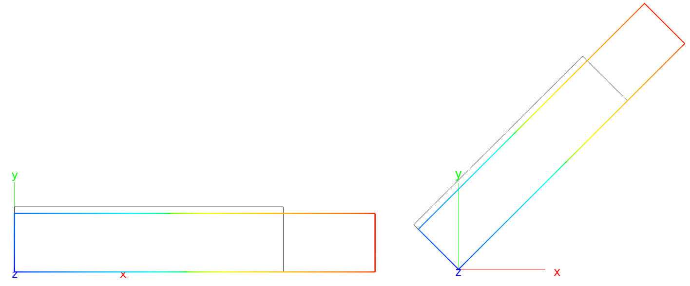
Deformed (colored) and undeformed (black) shapes. Left: Model (1), right: Model (2).

Results of model (2) are correct because of the correct mbase specification mbase 12 0 0 0 0 0 0 0 0 0:

• The material reference coordinate system is defined by angles of orientation (Euler angles) with respect to the element-local coordinate system (here: All Euler angles are 0, i.e that layer orientation is with respect to the element local system).

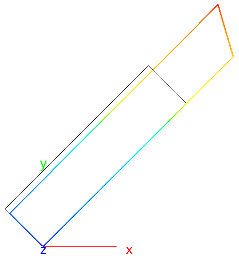
Deformed (colored) and undeformed (black) shapes of model (2). Results are wrong, because of the default mbase.

Note

Element stress and strain tensors are stored on the B2000++ model database with respect to the global coordinate system.

Mass and non-structural mass

B2000++ defines the non structural mass of rod, beam, ans shell elements

• in the property block for beam elements (Bx.S.RS). Reason: The Bx beam elements are the only B2000++ elements the define the element properties with the property block - similar to BDF, referring to pid (Nastran BDF defines the non structural mass in the element property cards, not in the element cards). Example definition non-structural mass:

  property 11
      type beam_section
      mid 1
      shape rectangle
      d1 0.01 d2 0.01
      non_structural_mass 0.27
  end
  

• in the element blocks for all other elements concerned. Reason: property blocks are not understood by these elements. Example definition non-structural mass:

  elements
      ...
      eltype Q4.S.MITC
      non_structural_mass 0.27
      ...
  end