All B2000++ deformation analysis elements are designed for static
and dynamic analysis, linear, material-nonlinear, and geometric
nonlinear analysis (a Total-Lagrangian approach is employed to account
for geometric nonlinearities).
The rod/cable elements are designed for static and dynamic, linear and
nonlinear analysis of truss and cable structures. The element topology
ist described in the Generic Element
section.
The Total-Lagrangian approach is employed to allow for arbitrary
rigid-body motions.
An initial strain, an initial stress, or an initial force can be
applied to rod and cable elements.
Axial stresses, strains, and forces stored on database are all
expressed in the element-local coordinate system. For nonlinear
analysis, the strain is the Green-Lagrange strain, while the stress is
the Cauchy stress. Axial stresses are stored in the
STRESS_SECTION_RODsampling point field
datasets. Axial strains are stored in the STRAIN_SECTION_ROD
datasets. Axial section forces are stored in the FORCE_SECTION_RODsampling point field datasets.
The R2.S is a two-node, fully-integrated rod/cable element. The shape
functions are compatible with the B2.S.RS beam element and with
the element edges of linear shell and continuum elements.
The R3.S is three-node, fully-integrated quadratic rod/cable
element. The shape functions are compatible with the B3.S.RS beam
element and with the element edges of quadratic shell and continuum
elements.
The R4.S is a four-node, fully-integrated cubic rod/cable element. The
shape functions are compatible with the B4.S beam element and with
the element edges of cubic shell and continuum elements.
Required MDL Parameters
midv
Specifies the element material number v (int) for all
subsequently specified elements. v remains valid until a new
mid parameters is encountered or until the element parameter
eltype is specified. Rod (cable) elements can process materials
of the following types: isotropic, viscoelastic
areat
Specifies the cross section area t (float). The same definition
will be used for all elements defined hereafter until a new area
parameter is encountered or until the element parameter eltype
is specified.
Optional MDL Parameters
initial_strain_xxv
Defines an initial strain e for subsequently defined beam
elements. The initial strain is assumed constant along the element
x-axis. The same definition will be used for all elements defined
hereafter, until a new initial_strain_xx parameter is
encountered or until the eltype command is specified.
initial_stress_xxv
Defines an initial stress s for subsequently defined beam
elements. The initial stress is assumed constant along the element
x-axis. The same definition will be used for all elements defined
hereafter, until a new initial_stress_xx parameter is
encountered or until the eltype command is specified.
initial_force_xv
Defines an initial force f acting at the centroid for
subsequently defined beam elements. The initial force is assumed
constant along the element x-axis. The same definition will be used
for all elements defined hereafter, until a new initial_force_x
parameter is encountered or until the eltype command is
specified.
initial_force_off_xfxmymz
Defines an initial force fx and an initial moment my (around
the local y-axis) and an initial moment mz (around the local
z-axis) acting at the Centroid of the section. The initial force and
the moments are assumed constant along the element x-axis. The same
definition will be used for all elements defined hereafter, until a
new initial_force_off_x parameter is encountered or until the
eltype command is specified.
groupgid
Defines the element group number gid (non-negative int). The
default group number is 0. The same definition will be used for all
elements defined hereafter, until a new group parameter is
encountered or until the eltype command is specified.
non_structural_massv or nsmv
Defines the non-structural mass per unit length. Default is 0. The
same definition will be used for all elements defined hereafter,
until a new non_structural_mass parameter is encountered or
until a new eltype command is specified.
The beam elements are designed for static and dynamic, linear and
nonlinear analysis. For nonlinear analysis, finite strains are
supported. The element topology is described in the Generic
Element section. Beam section-specific data are
described by the property MDL command. All other beam
data are described within the elements block and are
described below.
DOFs in global reference frame, F, M in element-local reference
frame.
Beam elements may contain an initial strain, stress, or force and
eccentricities. Special means for computing the cross-section
constants are available.
A two-node linear prismatic Timoshenko beam element with
selective under-integration, according to the Reissner/Simo
formulation. The shape functions are compatible with the
R2.S rod/cable element and with the element edges of linear
shell and continuum elements. This element may not be very
accurate for pure bending if only a single element is being
used to discretize a thin beam.
B3.S.RS
A three-node quadratic prismatic Timoshenko beam element with
selective under-integration, according to the Reissner/Simo
formulation. The shape functions are compatible with the
R3.S rod/cable element and with the element edges of
quadratic shell and continuum elements.
A two-node cubic Timoshenko beam element with 2*6
element-internal degrees-of-freedom. The shape functions are
not compatible with those of shell or solid elements, except at
the beam ends. A straight beam is assumed for the initial
configuration. Full integration is conducted with 5-point
Gauss-Legendre-Lobatto quadrature. Thus, stresses are
calculated also at the beam ends. This element is accurate for
pure bending. The behavior of a cubic Euler-Bernoulli beam
element can be achieved by setting the
shear_correction_factors in the beam property to a high
value.
B4.S
A four-node cubic Timoshenko beam element. The shape functions
are compatible with the R4.S rod/cable element and with the
element edges of cubic shell and continuum elements. Full
integration is conducted with 5-point Gauss-Legendre-Lobatto
quadrature. Thus, stresses are calculated also at the beam
ends. This element is accurate for pure-bending if it is not
curved in the initial configuration and if the nodes are
equidistant. The behavior of a cubic Euler-Bernoulli beam
element can be achieved by setting the
shear_correction_factors in the beam property to a high
value.
For linear analysis, the strains and stresses are the “engineering” stresses
and strains. For nonlinear analysis, the strain is the Green-Lagrange strain,
while the stress is the Cauchy stress.
Required MDL Parameters
beam_orientationxyz
Defines the beam orientation vector in the beam-local x-y plane. The
same definition will be used for all elements defined hereafter,
until a new beam_orientation parameter is encountered or until
the eltype command is re-specified.
beam_orientationrefnodev
Defines the (external) beam reference node v (positive int). The
reference node defines a vector in the beam local x-y plane together
with the first beam node. The same definition will be used for all
elements defined hereafter, until a new beam_orientation
parameter is encountered or until the eltype command is
specified. See also Generic Beam Elements for
the definition of the beam reference node.
pidv
Specifies the beam property identifier (positive int)
pointing to the beam property table. The same definition will be used for all
elements defined hereafter, until a new value v is encountered or until a
new element type is specified.
Note
non_structural_mass or nsm of Bx.S.RS elements must be
specified in the beam property block.
Optional MDL Parameters
beam_offsetsx1y1z1x2y2z2...
Defines the beam eccentricities (or offsets) for all nodes defining
the beam, for subsequently defined beam element. x, y, and
z are defined with respect to the branch reference frame. The
same definition will be used for all elements defined hereafter,
until a new beam_offsets parameter is encountered or until the
eltype command is specified. See also Generic Beam
Elements for the definition of the beam
eccentricities. Also see the description of the beam_section property for
an illustration
of beam offsets.
Warning
Applying beam_offsets to Reissner-Simo beam elements Bx.S.RS in a
geometrically nonlinear analysis with large rotations likely causes
convergence issues or failures in the current b2000++ version. Consider using
the section_offset
parameter instead, if the beam structure only needs to be offset to the
beam local x-axis in parallel.
beam_dof_release1pattern|clear
Release part of the element’s connections to the degrees-of-freedom
at the first node. The degrees-of-freedom to be released are
specified w.r.t. the beam-local coordinate system. pattern is a
concatenated string containing the degrees of freedom (1, 2, 3, 4,
5, or 6) to be released. clear removes all releases (i.e.,
nothing is released). The same definition will be used for all
elements defined hereafter, until a new beam_dof_release1
parameter is encountered or until the eltype command is
specified. Example:
beam_dof_release1 456
releases all rotational degrees of freedom.
beam_dof_release2pattern|clear
Release part of the element’s connections to the degrees-of-freedom
at the second node. The degrees-of-freedom to be released are
specified w.r.t. the beam-local coordinate system. pattern is a
concatenated string containing the degrees of freedom (1, 2, 3, 4,
5, or 6) to be released. clear removes all releases (i.e.,
nothing is released). The same definition will be used for all
elements defined hereafter, until a new beam_dof_release2
parameter is encountered or until the eltype command is
specified. Example:
beam_dof_release2 4
releases the rotational degree-of-freedom of the beam end node
around the beam-local x-direction (the beam axis).
initial_strain_xxv
Defines an initial strain e for subsequently defined beam
elements. The initial strain is assumed constant along the element
x-axis. The same definition will be used for all elements defined
hereafter, until a new initial_strain_xx parameter is
encountered or until the eltype command is specified.
initial_stress_xxv
Defines an initial stress s for subsequently defined beam
elements. The initial stress is assumed constant along the element
x-axis. The same definition will be used for all elements defined
hereafter, until a new initial_stress_xx parameter is
encountered or until the eltype command is specified.
initial_force_xv
Defines an initial force f acting at the centroid for
subsequently defined beam elements. The initial force is assumed
constant along the element x-axis. The same definition will be used
for all elements defined hereafter, until a new initial_force_x
parameter is encountered or until the eltype command is
specified.
Gradients (sampling point fields)
For beam elements, the b2000++ solver does not compute stresses and strains
directly. Instead, the stress resultants (section forces and section moments)
are evaluated at the integration points in the element-local coordinate system.
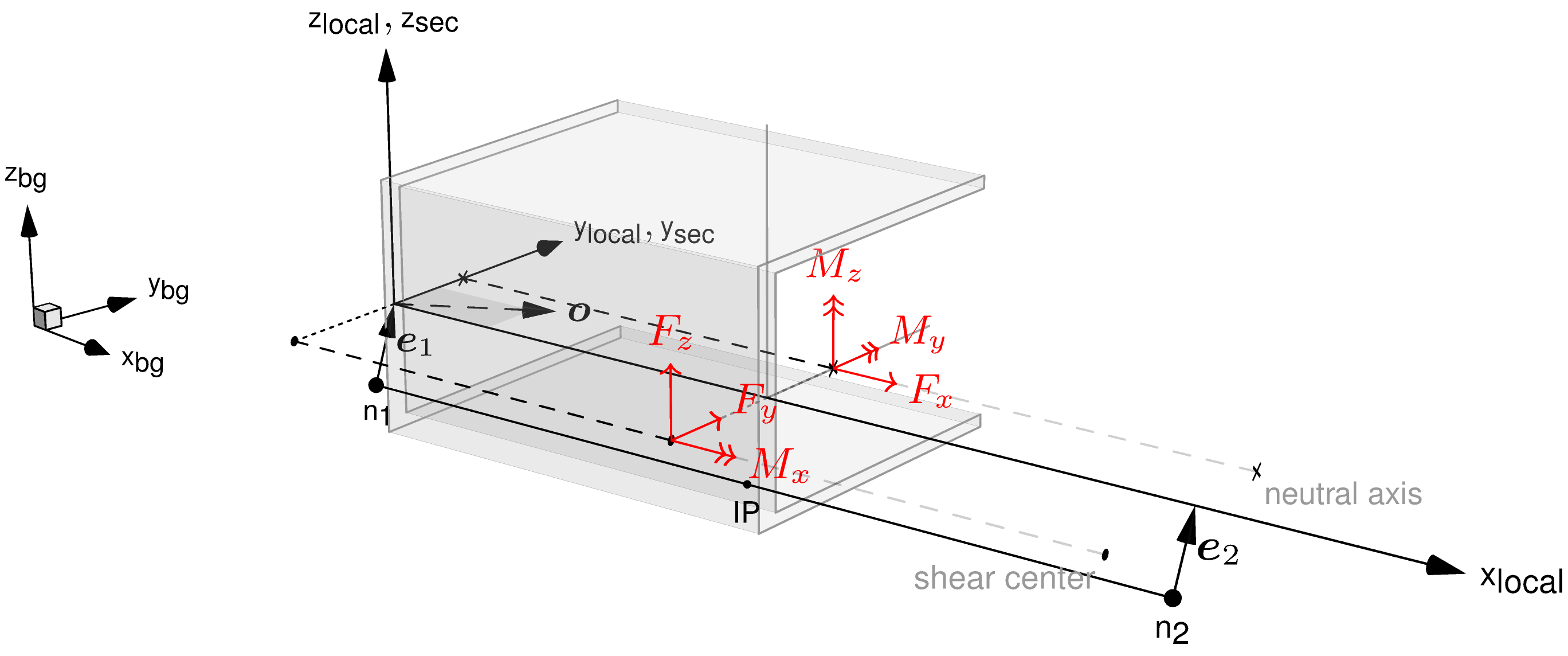
Specifically, the normal force \(F_x\) and bending moments \(M_y\),
\(M_z\) are evaluated at the centroid of the cross-section, while the shear
forces \(F_y\), \(F_z\) and torsional moment \(M_x\) are evaluated
at the shear center (see figure). They are stored in the
database under the keys FORCE_SECTION_BEAM
and MOMENT_SECTION_BEAM.
Section forces and moments at integration point IP of an B2.S.RS
element (nodes n1 and n2) with a C-shaped cross section,
beam_offsets vectors \(\mathbf{e}_1, \mathbf{e}_2\) and
beam_orientation vector \(\mathbf{o}\)
In a post-processing step, the section forces and moments can be extrapolated
from the integration points to the nodes. Recovery of the actual stress
distribution across the cross-section from these stress resultants can be
performed a posteriori with a tool such as the Simples bcs module or baspl++.
The shell elements are designed for static and dynamic, linear and
nonlinear analysis of thin- and thick-walled plate and shell
structures with isotropic, orthotropic and laminated, linear and
nonlinear materials. The element topology is described in the Generic
Element Section for triangular and
quadrilateral elements.
Like the Q4.S.MITC element, but with 4 incompatible modes for
in-plane bending.
The shell elements are based on Reissner-Mindlin shell theory and have
5 or 6 degrees of freedom per node. To account for geometric
nonlinearity, a Total-Lagrangian approach is employed. The MITC (Mixed
Interpolation of Tensorial Components) formulation (see [Bathe96],
[BatheMITC]) improves the out-of-plane behavior by interpolating the
through-the-thickness term of the strain tensor differently. This is a
better way for preventing out-of-plane locking than selective
under-integration. The rotation of the director is computed by making
use of finite rotations to allow for computing the director of the
deformed configuration directly by an algebraic expression of the
rotational degree of freedoms, i.e without numeric integration.
For laminates involving linear materials for all layers, the shell
elements automatically perform the through-the-thickness integration
a priori in analytical fashion. Hence, the number of layers is
irrelevant to the computation time of the first and second
variations. The benefit of this optimization is a considerable
speed-up for analysis of composite structures. Note that this
optimization does not alter the element response.
Stresses, strains, and any failure criteria which are stored in the
database, are computed at the integration points (“Gauss” points)
which are used by the element to compute the first and second
variations. The stresses and strains which are stored in the database
are all expressed in the branch global coordinate system. For linear
analysis, the strains and stresses stored in the database are the
“engineering” stresses and strains. For nonlinear analysis, the strain
is the Green-Lagrange strain, while the stress is the Cauchy stress.
The in-plane integration rule depends on the element type. For the
through-the-thickness integration, a 3-point Gauss-Legendre-Lobatto
rule is used (for laminates, this applies to each layer). This rule
ensures that gradients are evaluated at the surfaces and at the layer
boundaries, thus, where the maximum strains and stresses occur.
The Q9.S.MITC element is more effective (i.e. it has a better
ratio of accuracy vs. computational effort) than the other B2000++
shell elements, even for highly-distorted meshes. This element should
be considered whenever a new FE model is being made. The Q8.S.MITC
element is intended for FE models that were imported from other FE
codes that do not support nine-node quadrilateral elements.
Due to the incompatible modes, the Q4.S.MITC.E4 element does not
pass the patch tests (i.e. cannot exactly represent constant strain
fields), and it may exhibit instabilities in buckling analysis and in
nonlinear analysis. Elements of this type should not be significantly
distorted. While the in-plane bending response of this element is
better than the Q4.S.MITC element, the latter gives more
predictable results, especially concerning the gradients.
For the the quadratic MITC elements (T6.S.MITC, Q8.S.MITC,
Q9.S.MITC), mid-edge and mid-face nodes should be located at the
middle of the edges and centre of the face, respectively. Otherwise,
the Jacobian will contain higher-order terms, and the elements will
not work with full accuracy. However, for moderately curved geometries
such as cylindrical panels, the error is small enough that the
accuracy is still very good.
The T6.S.MITC element fails for certain double-curved geometries
such as hyperboloid shells. Further, for complex loading conditions,
this element may exhibit instabilities which affect the accuracy of
the linearized buckling load (i.e. the predicted buckling load will be
too low for coarse meshes).
Required MDL Parameters
midv
Specifies the element material number v (int) for all
subsequently specified elements. v remains valid until a new
mid parameters is encountered or until the element parameter
eltype is specified. Rod (cable) elements can process materials
of the following types: isotropic,
laminate, orthotropic, isotropic viscoelastic, orthotropic viscoelastic
nthicknesst1t2t3...
Specifies the element’s thickness at each of the element’s nodes.
This parameter allows to specify varying element thickness. The
element thickness is interpolated using the element’s in-plane shape
functions. Not required for laminate materials.
thicknesst
Specifies a constant element thickness t. Not required for
laminate materials.
Optional MDL Parameters
eccente
Defines the element eccentricity e, which is a constant offset of
the shell volume w.r.t. the shell reference surface. The same units
as for the coordinates and thicknesses are used. Default is 0. With
\(e = \frac{1}{2}t\), where t is the shell thickness, the shell
bottom surface coincides with the shell reference surface. With
\(e = - \frac{1}{2}t\), the shell top surface coincides with the
shell reference surface.
groupgid
Defines the element group number gid (non-negative int). The
default group number is 0. The same definition will be used for all
elements defined hereafter, until a new group parameter is
encountered or until the eltype command is specified.
morientationdefault
Resets to the default material orientation which is obtained by
projecting the branch-global x-direction onto the shell surface and
constructing an orthogonal reference frame (this will not work for
elements whose shell surface normal is aligned with the
x-direction).
morientation...end
Specifies the material orientation, see
morientation.
neccente1e2e3...
Defines the nodal eccentricities e (float), which are the offset
of the shell surface from the shell reference surface, at the nodal
position(s). This command allows to specify varying
eccentricity. The element eccentricity is interpolated using the
element’s in-plane shape functions. Otherwise, the definition is
similar to eccent.
non_structural_massv
Defines the non-structural mass per unit area. Default is 0. The
same definition will be used for all elements defined hereafter,
until a new non_structural_mass parameter is encountered or
until the eltype command is specified.
Optional MDL Parameters
drillsf
Defines the “drill” stiffness factor v (float) for shell element
nodes with 6 degrees-of-freedom and whose in-plane rotation (drill)
will be stabilized. Default is 1e-8. The effective drill stiffness
is calculated using the averaged in-plane shear modulus and the
element configuration and thickness, and is multiplied with
f. Hence, a value of 0 for f means no drill
stabilization. The section Shell Elements and the Drill
Stiffness contains additional information on the
problem of the drill stiffness.
drills applies only to the 6th degree of freedom of shell
elements that may need stabilization, in contrast to the autospc
parameter in conjunction with the (see MUMPS sparse linear
solver)
The two-dimensional elements support plane-stress and plane-strain
assumptions (whether the element will be used for plane-stress or
plane-strain analysis, must be indicated in the material
definition). Some elements support laminates. The mixed elements are
implemented according to [Sussman87] and [Bathe96] and can be
applied to quasi-incompressible materials.
Mixed formulation elements with linear internal pressure
field. They pass the inf-sup test.
Qx.S.2D.TL
Ux, Uy
Sxx, Syy, Szz, Sxy, Syz, Sxz
Exx, Eyy, Ezz, Exy, Eyz, Exz
Pure displacement formulation elements.
Q4.S.2D.E4
Ux, Uy
Sxx, Syy, Szz, Sxy, Syz, Sxz
Exx, Eyy, Ezz, Exy, Eyz, Exz
Enhanced-assumed strain (EAS) formulation with four
incompatible modes.
Qx.S.2D.UP1
Ux, Uy
Sxx, Syy, Szz, Sxy, Syz, Sxz
Exx, Eyy, Ezz, Exy, Eyz, Exz
Mixed formulation with constant internal pressure field. They do
not pass the inf-sup test.
Q9.S.2D.UP3
Ux, Uy
Sxx, Syy, Szz, Sxy, Syz, Sxz
Exx, Eyy, Ezz, Exy, Eyz, Exz
Mixed formulation elements with linear internal pressure
field. They pass the inf-sup test.
When using mixed elements with quasi-incompressible materials, the
global stiffness matrix becomes nearly non-definite. The default
sparse linear solver, dmumps, can handle such matrices, but other
sparse linear solvers may not work (see Sparse Linear Solvers
:ref:`eqsolvers).
Stresses, strains, and any failure criteria which are stored in the
database, are computed at the integration points (“Gauss” points)
which are used by the element to compute the first and second
variations. The stress and strain tensors stored in the database are
all expressed in the branch-global coordinate system. For linear
analysis, the strains and stresses stored in the database are the
“engineering” stresses and strains. For nonlinear analysis, the strain
is the Green-Lagrange strain, while the stress is the Cauchy stress.
The in-plane integration rule depends on the element type. For the
through-the-thickness integration, a 3-point Gauss-Legendre-Lobatto
rule is used (for laminates, this applies to each layer). This rule
ensures that gradients are evaluated at the surfaces and at the layer
boundaries, thus, where the maximum strains and stresses occur.
Required MDL Parameters
midv
Specifies the element material number v (int) for all
subsequently specified elements. v remains valid until a new
mid parameters is encountered or until the element parameter
eltype is specified. Rod (cable) elements can process materials
of the following types: isotropic,
laminate, orthotropic, isotropic viscoelastic, orthotropic viscoelastic
Optional MDL Parameters
groupgid
Defines the element group number gid (non-negative int). The
default group number is 0. The same definition will be used for all
elements defined hereafter, until a new group parameter is
encountered or until the eltype command is specified.
morientationdefault
Resets to the default material orientation which is obtained by
projecting the branch-global x-direction onto the shell surface and
constructing an orthogonal reference frame (this will not work for
elements whose shell surface normal is aligned with the
x-direction).
morientation...end
Specifies the material orientation, see
morientation.
The solid elements elements are designed for static and dynamic,
linear and nonlinear analysis of solids. The elements are formulated
with the Total Lagrangian formulation, see [Bathe96]. The element
topology ist described in the Generic Element Section for
tetrahedral, hexahedral, and prismatic
elements.
Enhanced-assumed strain (EAS) formulation with nine
incompatible modes. Supports laminates.
HE8.S.UP1
Ux, Uy, Uz
Sxx, Syy, Szz, Sxy, Syz, Sxz
Exx, Eyy, Ezz, Exy, Eyz, Exz
Mixed formulation with constant internal pressure field. Does
not pass the inf-sup test.
HE20.S.UP1
Ux, Uy, Uz
Sxx, Syy, Szz, Sxy, Syz, Sxz
Exx, Eyy, Ezz, Exy, Eyz, Exz
Mixed formulation with constant internal pressure field. Passes
the inf-sup test.
HE27.S.UP4
Ux, Uy, Uz
Sxx, Syy, Szz, Sxy, Syz, Sxz
Exx, Eyy, Ezz, Exy, Eyz, Exz
Mixed formulation with linear internal pressure field. Passes
the inf-sup test.
All solid elements support isotropic, orthotropic and also layered
materials. For laminates involving linear materials for all layers,
the shell elements automatically perform the through-the-thickness
integration once in an analysis.
All elements are isoparametric. The nodal degrees-of-freedom are the
displacements. All elements pass the MacNeal-Harder patch test (i.e.
they can represent a constant strain field exactly).
HE8.S.E9 elements may exhibit instabilities in nonlinear analysis,
due to the incompatible modes. Elements of these types should not be
significantly distorted.
When using mixed elements with quasi-incompressible materials, the
global stiffness matrix becomes nearly non-definite. The default
sparse linear solver, dmumps, can handle such matrices, but other
sparse linear solvers may not work (see Sparse Linear Solvers
:ref:`eqsolvers).
Stresses, strains, and any failure criteria which are stored in the
database, are computed at the integration points (“Gauss” points)
which are used by the element to compute the first and second
variations. The stresses and strains which are stored in the database
are all expressed in the branch global coordinate system. For linear
analysis, the strains and stresses stored in the database are the
“engineering” stresses and strains. For nonlinear analysis, the strain
is the Green-Lagrange strain, while the stress is the Cauchy stress.
The in-plane integration rule depends on the element type. For the
through-the-thickness integration, a 3-point Gauss-Legendre-Lobatto
rule is used (for laminates, this applies to each layer). This rule
ensures that gradients are evaluated at the surfaces and at the layer
boundaries, thus, where the maximum strains and stresses occur.
Required MDL Parameters
midv
Specifies the element material number v (int) for all
subsequently specified elements. v remains valid until a new
mid parameters is encountered or until the element parameter
eltype is specified. Rod (cable) elements can process materials
of the following types: isotropic,
laminate, orthotropic, isotropic viscoelastic, orthotropic viscoelastic
Optional MDL Parameters
groupgid
Defines the element group number gid (non-negative int). The
default group number is 0. The same definition will be used for all
elements defined hereafter, until a new group parameter is
encountered or until the eltype command is specified.
morientationdefault
Resets to the default material orientation which is obtained by
projecting the branch-global x-direction onto the shell surface and
constructing an orthogonal reference frame (this will not work for
elements whose shell surface normal is aligned with the
x-direction).
morientation...end
Specifies the material orientation, see
morientation.
The axisymmetric elements are designed for static linear analysis of solids that possess rotational
symmetry about the global y-axis. It is ideal for thick‑walled cylinders, pipes, pressure vessels, and other axis‑symmetric geometries under internal/external pressure, axial loading, or radial thermal gradients.
The elements are formulated with the Total Lagrangian formulation, see [Bathe96]. The element
topology is coincident with those described in the Generic
Element Section for triangular and
quadrilateral elements.
Theoretically speaking, axisymmetric elements and its physical result properties such as deformation
rely on a cylindrical coordinate system definition. Each point in cylindrical space can be described
by a vector (r,t,z) of length 3. Since there is no such explicit coordinate system
definition in B2000++, all nodes as part of an axisymmetric model need to be defined in an ordinary
cartesian space which is to be intepreted to the desired axisymmetric geometry accordingly.
By definition, the mapping between cartesian and cylindrical coordinates in B2000++ is the following:
The first coordinate (x-axis) maps to the radial coordinate (x -> r)
The second coordinate (y-axis) maps to the local axial coordinate (y -> z)
The third coordinate (z-axis) maps to the local tangential coordinate (z -> t) is ignored due to symmetry
(NOTE: at least a “0” must be present because B2000++ requires points in 3D!)
Stresses and strains
Stresses, strains which are stored in the database, are computed at the integration points (“Gauss” points) which are used by the element to compute the first and second variations.
The stresses and strains which are stored in the database are all expressed in the branch global coordinate system.
Relying on a pure two-dimensional element formulation, all shear strains with respect to the tangential coordinate vanish.
Required MDL Parameters
midv
Specifies the element material number v (int) for all
subsequently specified elements. v remains valid until a new
mid parameters is encountered or until the element parameter
eltype is specified. Axisymmetric elements can process materials
of the following types: isotropic,
orthotropic
A simple two element example on how to define axisymmetric elements
is given below with the corresponding graphical representation.
A point mass element defines masses and mass moments of inertia at a
mesh node, with respect to the node-local coordinate system, see
transformations and nodes commands.
For static analysis the point masses will be used to compute inertia
forces.
For dynamic analysis point mass will be added to the global mass
matrix.
The point mass elements PMASS3.S and PMASS6.S work for linear and
geometric nonlinear analysis.analysis.
Adds mass forces to 3 translational DOFs and mass moments to
the 3 rotation DOFs of a node.
Required MDL Parameters
massm
Specifies the ‘lumped’ nodal mass m (float) of PMASS3.S and
PMASS6.S elements. mass remains defined until a new mass
parameter is specified or until a new eltype parameter is
specified.
Specifies the coefficients of the symmetric nodal mass coefficient
matrix, i.e the 21 terms stored column-wise (upper triangle of
matrix) of PMASS6.S elements. If matrix is specified, mass,
inertia_moments, and offsets may not be specified, and vice
versa.
inertia_momentsIxxIyyIzzIxyIyzIxz
Specifies the components of the inertia moment tensor, expressed in
the branch-global coordinate system (PMASS6.S ements). The inertia
moments are 0 by default.
offsetsoxoyoz
Specifies the offset, in each direction, of the mass point with
respect to the node (PMASS6.S elements). The default offset
\(o\) in each direction is 0.
Optional MDL Parameters
groupgid
Defines the element group number gid (non-negative int). The
default group number is 0. The same definition will be used for all
elements defined hereafter, until a new group parameter is
encountered or until the eltype command is specified.
Mass Matrix
The mass matrix is computed as follows for a PMASS6.S element:
Define masses of 10000 in each of the three translation directions for
node 45 and 230 and masses of 50000 each of the three translation
directions for node 457 (note the PMASS3.S element identifiers are 1,
2, and 3, respectively):
elements
   eltype pmass3.s
   mass 10000
   1 45
   2 230
   mass 50000
   3 457
end
The “rigid-body” element couples the displacement and the rotational
degrees-of-freedom of one or several slave nodes with the
displacement and rotational degrees-of-freedom of the master node in
such a way that this corresponds to a rigid-body motion.
Because the number of connected nodes is not fixed, the element
connectivity has to be enclosed by square brackets “[” and “]”. The
master node is specified first, followed by the slave nodes. For
mesh-independent definitions, the slave nodes can be specified by
means of nodesets.
MDL Specification
elements
    ...
    type RBE
    element-id [ n0 (dof pattern) n1 n2 ... ]
    element-id [ n0 (dof pattern) nodeset nid ]
    element-id [ n0 (dof pattern) epatch epatch-id e1-e12|f1-f7|b ]
    ...
end
The degrees-of-freedom of the slave nodes to be coupled can be
specified by means of the optional dof parameter, where
pattern specifies the degrees-of-freedom in the form of digits
1-6, corresponding to the Ux, Uy, Uz, Rx, Ry, Rz
degrees-of-freedom. For example, 123 means all displacement
degrees-of-freedom, and 123456 means all displacement and rotation
degrees-of-freedom. The default 123456 will be applied, unless
dof is specified. Once set, the specified degrees-of-freedom will
be applied to any subsequent slave nodes until a new dof parameter
is given.
Example
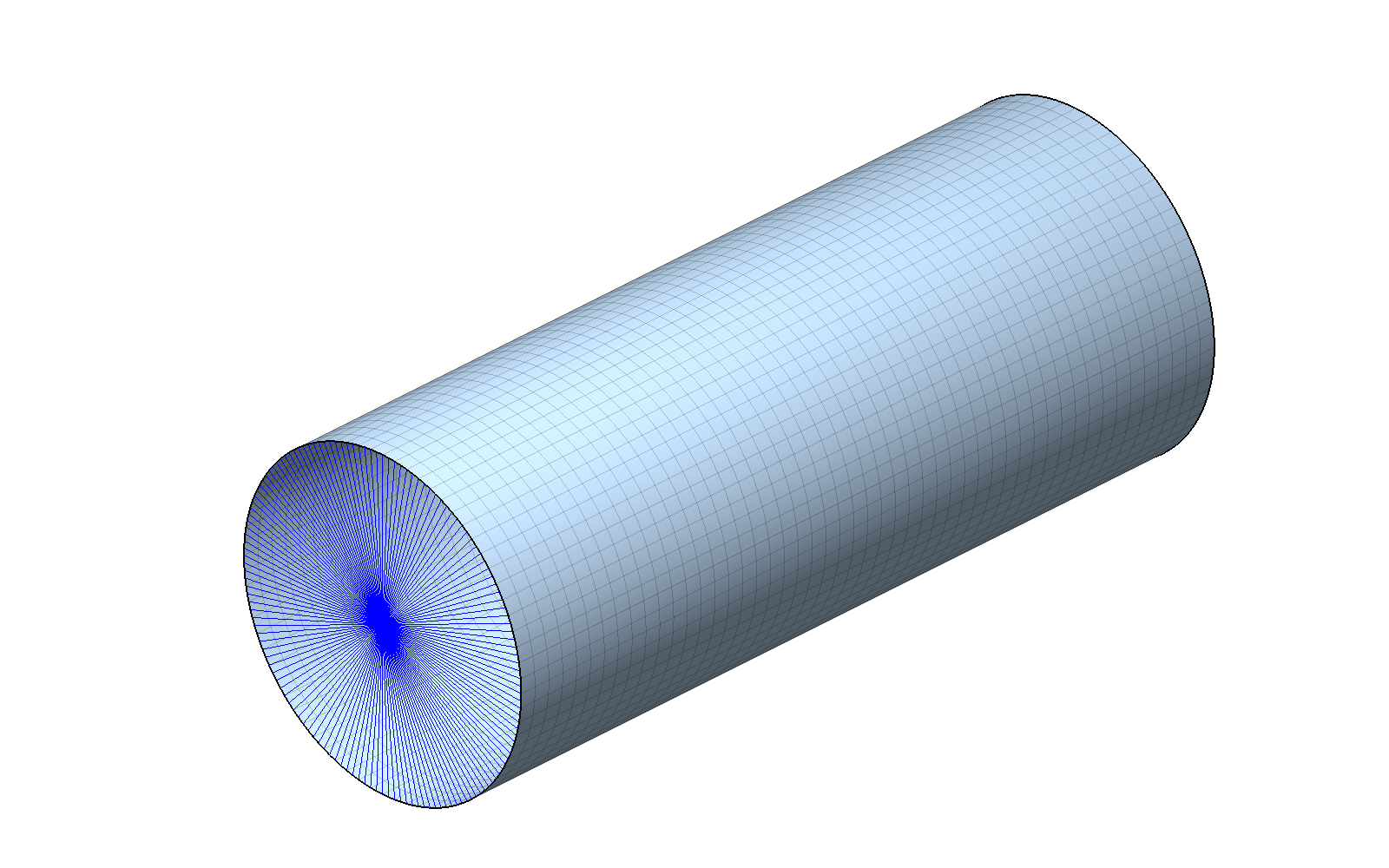
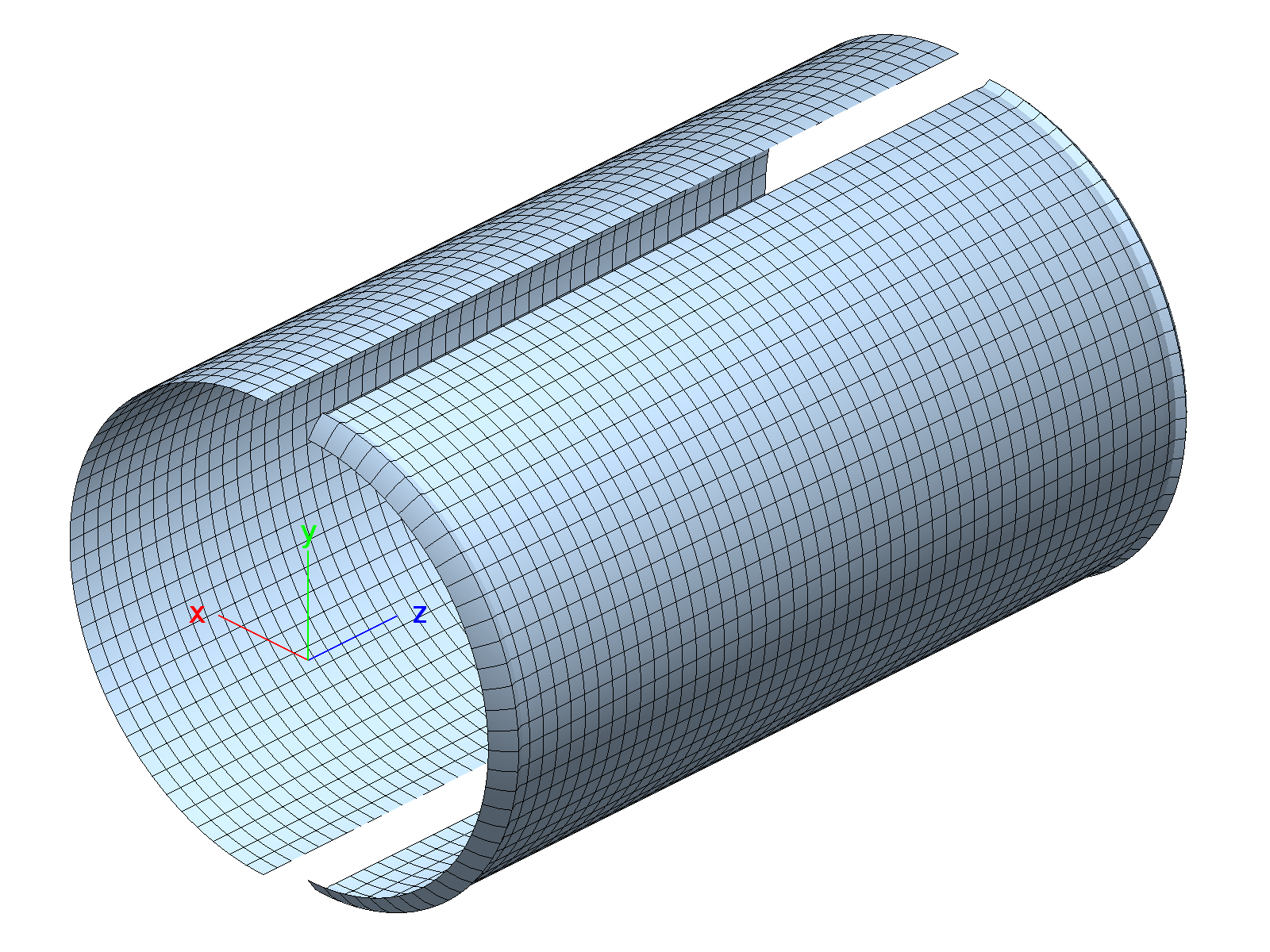
This example demonstrates the use of dof and of node sets. A
cylindrical shell made of aluminum with a radius of 2 m , a length of
10 m and a thickness of 2.5 mm is clamped at one end and shall be
subjected to a bending force applied at the other end. The axis of the
cylinder coincides with the z-direction. Both ends are connected to an
RBE element. One end is fixed (condition ebc1), while an axial
force is applied to the other end (condition nbc1).
Note that the epatch command is used to generate a
cylindrical mesh, here with Q9.S.MITC shell elements. The parameter
localall generates local reference frames (cylindrical
coordinates) for all nodes, with the first direction aligned with the
radial direction.
With the above definition the nodes move freely in the radial
direction. Alternatively, the RBE elements can be specified such that
the radial displacements of the slaves are fixed:
The displacement field is compared for the two models in the following
figure.
Axially-compressed cylinder (linear analysis, deformations are
amplified). Left: The radial displacement DOFs are not coupled.
Right: All slave DOFs are coupled.
The element is linear and works with the branch-global coordinate
system, i.e., it ignores any node-local coordinate systems. If only
one degree-of-freedom is specified, this will be connected to the
ground:
\[F = Ku_{1} + Dv_{1}\]
If a translation degree-of-freedom (Ux, Uy, or Uz) is specified, that
node will have 3 degrees-of-freedom. If a rotation degree-of-freedom
(Rx, Ry, or Rz) is specified, that node will have 6
degrees-of-freedom. In this case it may be necessary to lock the
degrees-of-freedom that are not connected.
If a node-local coordinate system is defined on the node, and systemlocal is specified, the spring translation or rotation is in that
node-local coordinate system.
MDL Specification
 elements
     type SPRING
     element-id [ K kcoeff (D dcoeff) node n1 dof dof1 (system branch|local)]
     element-id [ K kcoeff (D dcoeff) node n1 dof dof1 (system branch|local) node n2 dof dof2 (system branch|local)]
 end

The element stiffness K (float) must be specified. The damping
coefficient D is optional and has a default value of 0.
Example
Two spring elements connect degrees-of-freedom Ux (translation in
X-direction) and Ry (rotation around the Y-axis) of node 1 to the
ground. No damping coefficients are specified, thus, the default value
of zero will be used. There is also a point-mass element defined at
that node. The node could be connected by an RBE element to other
parts of a FE model. This is not the case here, therefore, the
degrees-of-freedom not connected are locked.
The distributed coupling element connects the degrees-of-freedom at a
slave node with those at one or several master nodes, according to the
master node weights. Which degrees-of-freedom (DOF) are coupled,
depends on the DOF specification.
Because the number of connected nodes is not fixed, the element
connectivity has to be enclosed by square brackets […]. The slave
node identifier ns (int) is specified first, followed by one or
more master node identifiers mn (int). For mesh-independent
definitions, the master nodes can be specified by means of
nodesets.
MDL Specification
elements
  type FMDE
  element-id [ (dof v) ns mn1 mn2 ... ]
  ...
end
The master nodes list can consist of individual node identifiers,
optionally preceded by a weight assigned to a master node:
(weight w1) mn1 (weight w2) mn2 ...
Master nodes can be specified with one or more nodesets:
(weight w) nodeset id
where id is the nodeset name (string). Master nodes can be also
specified with one or more epatch edge, face
or body node lists:
(weight w) epatch id e1-e12|f1-f7|b
where id is the epatch identifier (int), ex an edge number,
fx a face number, and b the body (all nodes).
The degrees-of-freedom to be coupled can be specified by means of the
dof parameter. It takes an integer number v which contains the
digits 1-6, corresponding to the Ux, Uy, Uz, Rx, Ry, Rz
degrees-of-freedom. For example, 123 means all displacement
degrees-of-freedom, and 123456 (default) means all displacement and
rotation degrees-of-freedom.
If a weight w (float) is specified (default is 1.0), it will be
applied to any subsequent master nodes until a new weight is
specified.
Shell-to-solid coupling (SSC) elements couple discontinuous shell and
solid meshes. In this case the interpolated displacements between
shell and solid elements cannot be made wholly continuous. For this
reason, the goal is to minimize the difference rather than to
eliminate it.
This scenario is typically found in global-local analyses where the
global part of the model consists of shell elements while the local
part consists of solid elements. Usually, the local part is meshed
much finer.
This section describes the SSC elements and how they can be generated
automatically.
Alternatively, the field_transfer method can be
employed for shell-to-solid coupling. While the SSC elements
constitute a point-wise coupling, field_transfer
performs a weighted-residual coupling.
Requirements and implementation
In addition to different element sizes and node positions, the
shell-to-solid coupling must also account for the transformation of
the rotational degrees-of-freedom of the shell elements to the
translation degrees-of-freedom of the connected solid elements. This
coupling depends on how the shell element directors are calculated
from the degrees-of-freedom, a procedure which is specific to the
shell element’s formulation and implementation. Hence, the
shell-to-solid coupling must be tailor-made for each type of shell
element.
In geometrically nonlinear analysis, large rigid-body motions may
occur. The shell-to-solid coupling must be performed such that the
coupling between the degrees-of-freedom is performed taking into
account the current (rotated) configuration. Hence, a linear approach
such as enforcing minimal displacement discontinuity by means of the
linc will fail.
For these reasons, shell-to-solid coupling in B2000++ is implemented
in the form of Finite Elements which (a) are specifically made for
each supported shell element type, and (b) support geometrically
nonlinear analysis. This allows for incorporating the coupling in the
standard solution procedures involving the computation of the first
and second variation.
The shell-to-solid coupling elements for the MITC shell elements in B2000++ enforce their constraints using
B2000++’s constraint system. By default, the Augmented Lagrange method
is used for the static linear and nonlinear solvers, and the Lagrange
method is used for the dynamic nonlinear solver. See
Linear and Nonlinear Constraint Control for details.
Automatic definition of SSC elements
When the add_ssc_elements parameter is specified in the
adir command the B2000++ input processor b2ip++`
will automatically add the necessary SSC elements. In that case the
explicit definition of SSC elements in the MDL file is not
necessary. Example:
adir
  case 1
  add_ssc_elements
end
The criteria defining when and how these elements are added are based
on the evaluation of geometrical properties; in particular, the volume
element’s node must lie (within sufficient tolerance) in the plane
defined by the shell element’s edge. Thus, this automatic procedure is
limited to straight and moderately curved shell elements.
Instead of having the SSC elements added automatically, the SSC
elements also can be specified explicitly in the MDL file. This is
described in the following.
SSC element connectivity
The shell-to-solid coupling elements are rigid and have no materials
associated to them. They connect a single edge of a shell element with
a single node of 3D solid element. Hence, all nodes of all adjacent
solid element’s faces must have a separate coupling element
associated.
In the above figure, a shell element defined by nodes \(n_1, n_2,
n_3, n_4\) is to be linked to a solid element face defined by nodes
\(a, b, c, d\). The link is defined such that the solid element
face (green) deforms in the same plane as the shell edge (defined by
nodes \(n_1, n_2\) in the above figure), the shell edge deforming
according to the shell node directors (dashed blue lines). Thus, for
the above configuration, 4 coupling elements must be defined, each of
them connecting the shell nodes \(n_1, n_2, n_3, n_4\) to one of
the solid face nodes 1-4:
\begin{equation}
\begin{bmatrix}
n_1 & n_2 & n_3 & n_4 & a
n_1 & n_2 & n_3 & n_4 & b
n_1 & n_2 & n_3 & n_4 & c
n_1 & n_2 & n_3 & n_4 & d
\end{bmatrix}
\end{equation}
The element node connectivity sequences of all coupling elements are
specified with first specifying the N nodes defining the shell followed
by one of the solid element nodes k:
n1n2...nNk
n1 to nN are the nodes defining the shell element according to
the element connectivity definition of the specific shell element,
with the following modification: n1 and n2 are nodes
defining the shell element edge to be coupled to the solid. This
means that in some cases the original shell element connectivity and
the connectivity can be permuted! k is the k-th element node
connectivity index of the solid element involved in the coupling
process.
Shell-to-solid coupling element linking a T3.S.MITC triangular
shell element to a single node of a 3D solid element. The solid
element node will deform with the edge of the shell element
defined by the first 2 nodes in the element connectivity list.
SSC.T6.S.MITC
Shell-to-solid coupling element linking a T6.S.MITC
second-order triangular shell element to a single node of a 3D
solid element. The solid element node will deform with the edge
of the shell element defined by the first 2 nodes in the
element connectivity list.
SSC.Q4.S.MITC
Shell-to-solid coupling element linking a Q4.S.MITC
quadrilateral shell element to a single node of a 3D solid
element. The solid element node will deform with the edge of
the shell element defined by the first 2 nodes in the element
connectivity list.
SSC.Q8.S.MITC
Shell-to-solid coupling element linking a Q8.S.MITC
second-order quadrilateral shell element to a single node of a
3D solid element. The solid element node will deform with the
edge of the shell element defined by the first 2 nodes in the
element connectivity list.
SSC.Q9.S.MITC
Shell-to-solid coupling element linking a Q9.S.MITC
second-order quadrilateral shell element to a single node of a
3D solid element. The solid element node will deform with the
edge of the shell element defined by the first 2 nodes in the
element connectivity list.
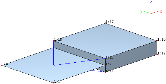
Example of SSC definition in the MDL file
The following simple example demonstrates how SSC elements can be
used. It consists of a single quadrilateral shell element which is to
be connected to a single hexahedral solid element. The thickness of
the shell element is equal to that of the solid element, and the
positions in the x- and y-direction at the interface coincide. Note
that this is not required, there may be multiple solid elements in the
thickness and also multiple solid elements in the y-direction.
The SSC elements are displayed as blue lines going from the node of the
3D solid element to the center of the shell element.
Th heat transfer analysis elements allow for solving linear,
nonlinear, stationary and non-stationary heat transfer problems.
Note
Heat transfer elements and deformation analysis elements cannot be
mixed in a single case. Coupled heat analysis and
deformation analysis problems must be solver separately, with a
staggered scheme.
All heat conduction elements are isoparametric. The degrees-of-freedom
are the temperatures at the element nodes. The gradients are the heat
fluxes in the global x- and y-direction.
Specifies the element material number v (int). The referenced
material must be of type `heat.
Optional MDL Parameters
groupgid
Defines the element group number gid (non-negative int). The
default group number is 0. The same definition will be used for all
elements defined hereafter, until a new group parameter is
encountered or until the eltype command is specified.
All heat conduction elements are isoparametric. The degrees-of-freedom
are the temperatures at the element nodes. The gradients are the heat
fluxes in the global x-, y-, and z-direction.
Required MDL Parameters
midv
Specifies the element material number v (int). The referenced
material must be of type `heat.
Optional MDL Parameters
groupgid
Defines the element group number gid (non-negative int). The
default group number is 0. The same definition will be used for all
elements defined hereafter, until a new group parameter is
encountered or until the eltype command is specified.
The one-dimensional wire elements and the two-dimensional surface
elements for specifying convection and radiation conditions
(von Neumann conditions) are ‘overlay’ elements, i.e. they are added
to edges or faces of heat conduction element and they do not have own
degrees of freedom. All convection and radiation elements are
isoparametric.
One-dimensional Heat Convection and Heat Radiation Overlay Elements
Element Name
Description
Lx.HEAT.RADCONV
Line elements, x=2,3
Required MDL Parameters
midv
Specifies the element material number v (int). The referenced
material must be of type `heat.
Optional MDL Parameters
groupgid
Defines the element group number gid (non-negative int). The
default group number is 0. The same definition will be used for all
elements defined hereafter, until a new group parameter is
encountered or until the eltype command is specified.
Heat Convection and Heat Radiation Overlay Elements
Element Name
Description
Lx.HEAT.RADCONV
Line elements, x=2,3
Tx.HEAT.RADCONV
Triangular elements, x=3,6,7
Qx.HEAT.RADCONV
Quadrilateral elements, x=4,8,9
Required MDL Parameters
midv
Specifies the element material number v (int). The referenced
material must be of type `heat.
Optional MDL Parameters
groupgid
Defines the element group number gid (non-negative int). The
default group number is 0. The same definition will be used for all
elements defined hereafter, until a new group parameter is
encountered or until the eltype command is specified.
The element material orientation specification of MDL defines the
orientation of materials with respect to references systems. There are
two methods for defining the material orientation:
morientation: Specifies the element material
orientation.
mbase: Specifies the material base (“old”
method, deprecated).
morientation specifies the material orientation. This
can be done in one of several ways. The morientation command is
specified in the MDL elements block.
MDL Specification
morientation
   parameters
end
The first way is to specify a base with two vectors, from which an
orthogonal reference frame is constructed (the base specified base
vectors do not need to be orthogonal, but they must not be co-linear).
The following operations are optional: The reference frame can be
rotated about one of its axes. One of the axes can then be projected
onto the element reference surface to construct an orthogonal
reference frame whose Z-axis is aligned with the element normal.
Finally, the reference frame can be rotated again about its Z-axis:
morientation
    base u1 u2 u3  v1 v2 v3
    rotate axis X|Y|Z angle a # optional
    project axis X|Y|Z]  # optional
    rotate angle a # optional
end
The second way specifies a transformation, from which an orthogonal reference frame for
the coordinates of the element integration point is calculated. The
following operations are optional: The reference frame can be rotated
about one of its axes. One of the axes can then be projected onto the
element reference surface to construct an orthogonal reference frame
whose Z-axis is aligned with the element normal. Finally, the
reference frame can be rotated again about its Z-axis:
morientation
    transformation id
    rotate axis X|Y|Z angle a # optional
    project axis X|Y|Z # optional
    rotate angle a # optional
end
The third way specifies a vector which is projected onto the reference
surface (which is defined by the element-local X- and Y-axes), to
construct an orthogonal reference frame whose Z-axis is aligned with
the element-local Z-axis. This reference frame can then be rotated
about the Z-axis:
morientation
    vector u1 u2 u3
    rotate angle a # optional
end
Another possibility is to use the element-local reference frame as
calculated at the element integration point. This reference frame can
be rotated about the Z-axis:
morientation
    element
    rotate angle a # optional
end
The rotation angles are specified in degrees. When using laminate
materials, a final rotation about the ply angle performed
automatically. For the projection, it is necessary that the projected
axis or vector is not co-linear with the shell surface normal.
To visualize the material orientations as calculated at the element
integration points, an analysis (for example linear) must be performed
with the gradients parameter set
to 1. This will write the dataset MBASE_IP to the database which
can be visualized with baspl++ usig the following script:
The material reference coordinate system is identical to the
branch coordinate system. The base vectors e11e12e13e21e22e23e31e32e33 are then dummy vectors, but must be
specified with dummy float values.
1
Thematerial reference coordinate system is defined by base
vectors e11e12e13e21e22e23e31e32e33 with respect
to the branch coordinate system.
2
The material reference coordinate system is defined by base
vectors e11e12e13e21e22e23e31e32e33 with respect
to the element-local coordinate system.
3
The material reference coordinate system is defined by base
vectors e11e12e13e21e22e23e31e32e33 with respect
to the integration point local coordinate system.
12
The material reference coordinate system is defined by angles
of orientation (Euler angles) e11e12e13 with respect to
the element-local coordinate system. The remaining values
e21e22e23e31e32e33 are then dummy values, but must be
specified with dummy float values.
13
The material reference coordinate system is defined by angles
of orientation (Euler angles) e11e12e13 with respect to
the integration point local coordinate system. The remaining
values e21e22e23e31e32e33 are then dummy values, but
must be specified with dummy float values. Note that the
default element material reference coordinate system is
element-dependent, see Generic Elements.
All B2000++ elements requiring numerical integration have a built-in
default integration rule. The default integration rule can be changed
with the ischeme element parameter.
The type of integration rule depends on the element type (for example,
integration rules for triangles cannot be applied to quadrilateral
elements). The command ischemedefault sets the default
integration rule.
Optional MDL Parameters
ischemetype
Specifies the integration rule to be selected for subsequently
specified elements. An appropriate integration rule is chosen by
default, which can be overridden by ischeme. type is one
of:
default
Resets the integration scheme to the default value for the
selected element type.
TETRAn
Integration rule for tetrahedral elements, where the integration
order n is one of 1, 2, 3, 4, 5, 6, and designates the
maximum order to which monomials can be integrated exactly:
\[\iiint x^{a}y^{b}z^{c} dx dy dz\quad;\quad a + b + c \leq o\]
The number of integration points is 1, 4, 5, 14, 15, 24,
respectively.
GAUSSn1[Xn2[Xn3]] | GLLn1[Xn2[Xn3]]
n1*n2*n3 point Gauss-Legendre or Gauss-Legendre-Lobatto
tensor-product integration rules for line elements,
quadrilateral elements, and hexahedral elements,
respectively. n1, n2, and n3 (1-32) define the
maximum order of integration in each element’s element-internal
direction \(o_{i} = 2n_{i} - 1\) and \(o_{i} = 2n_{i} -
3\) for Gauss-Legendre and Gauss-Legendre-Lobatto, respectively.
Due to the limited numerical precision of the 64bit CPUs (15-16
decimal places), Gauss-Legendre and Gauss-Legendre-Lobatto
integration rules with 1 greater than 15 are inaccurate, the
error increasing with the number of integration points.
TRIANGo_GAUSSx and TRIANGo_GLLn
Tensor-product integration rule for prism elements, where x
is one of 1-20 and designates the order to which monomials can be
integrated exactly in-plane, and n is the number of
integration points for the GAUSS or GLL rule in vertical
direction.
Example
Define 3 by 3 Gauss integration rule for element 1 and a 4 by 4
Gauss-Legendre-Lobatto rule for element 2. Element is reset to the
default rule.