2. Solid Mechanics
2.1. Static Analysis
2.1.1. Deformation Analysis of a Bolt
Location of case: $B2VERIFICATION/solid_mechanics/static/bolt
The deformations and the stresses of a bolt under external mechanical loading are computed (linear elastic analysis). The example case FE model is a 3-dimensional (solid) model consisting of quadratic isoparametric elements, i.e. HE20 hexahedral, TE10 tetrahedral, and PY15 prismatic elements.
The model originates from a study performed at the NLR
(1995). Originally generated for an analysis with Nastran (c) mesher,
the model has been converted to B2000 MDL input format. The model
exhibits about 150000 degrees of freedom. The figure below displays
the surface mesh (obtained with the baspl++ script
bv-mesh-and-bc.py):
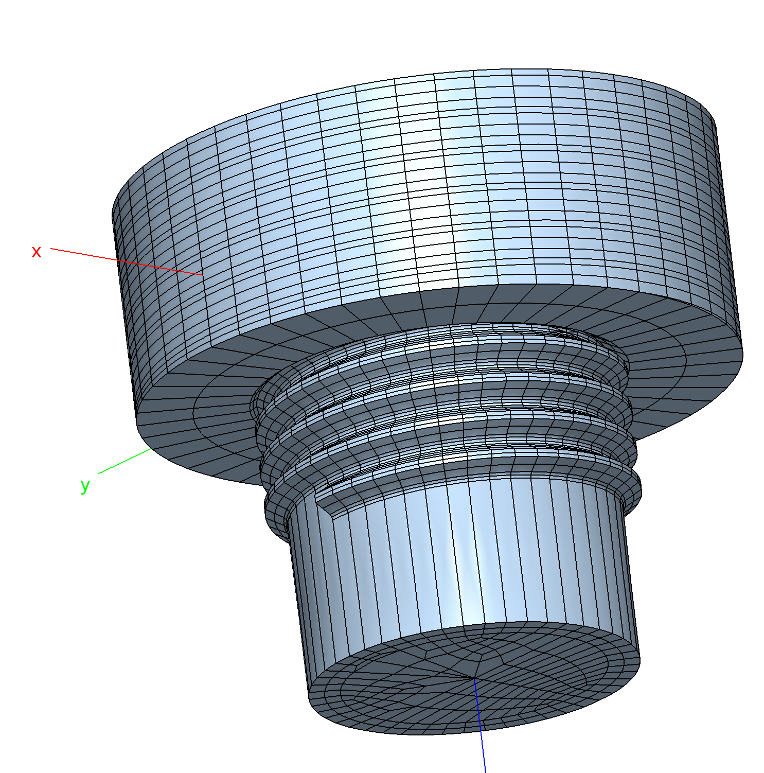
Bolt: Mesh and constrained nodes in x-y plane (red).
The bold is pulled by a surface traction load of \(t_z=100\) in the x-y plane of \(z=z_{max}\). With a radius of 5.2 the sum of applied forces in z is \(F_z=8457\) versus \(F_z=8495\) (B2000++).
Deformations and stresses are produced with the baspl++ scripts
bv-deformed.py (deformation plot) and bv-stress.py (von Mises
comparison stress).
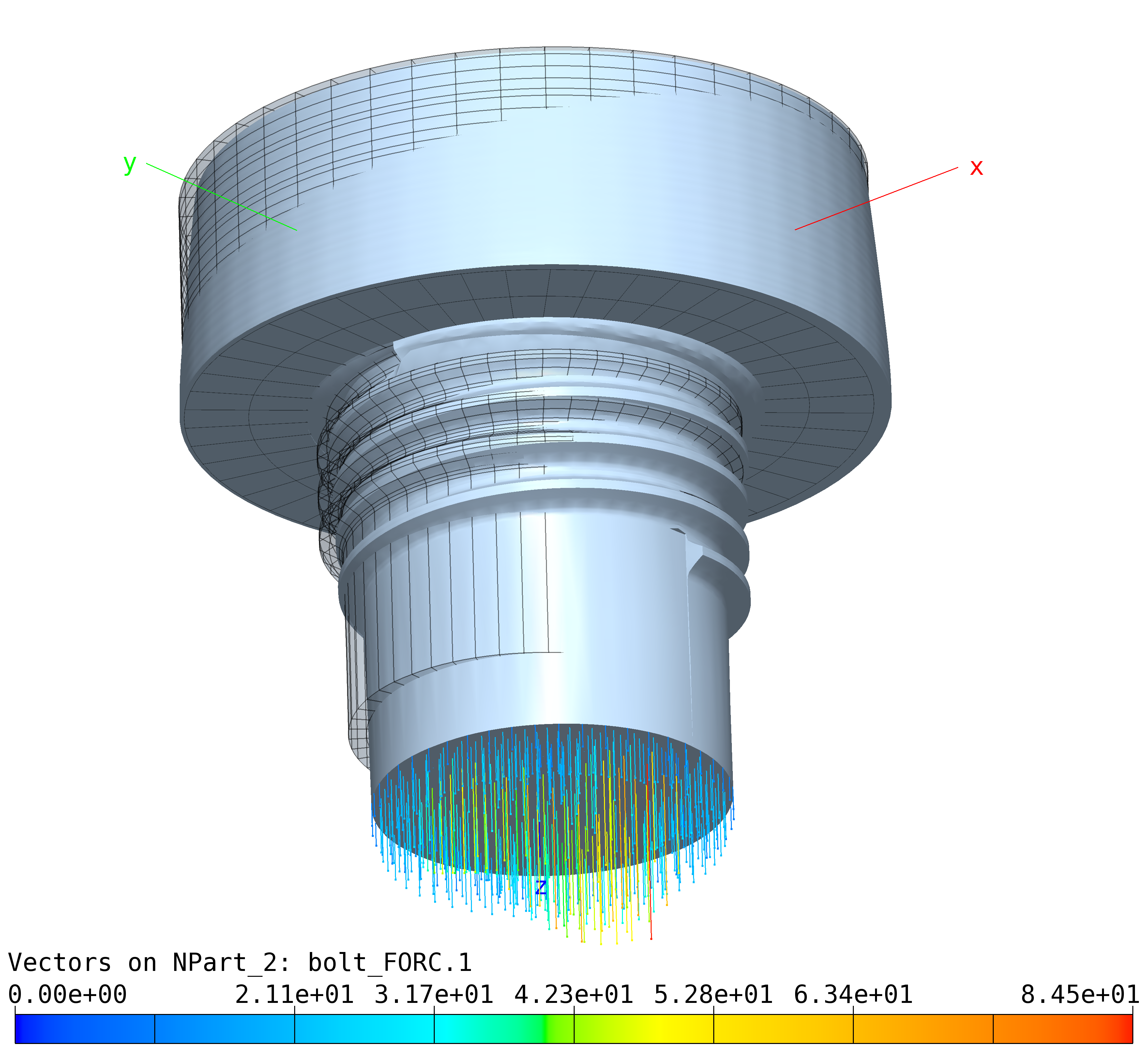
Bolt: Deformed mesh and mechanical forces generated by B2000++.
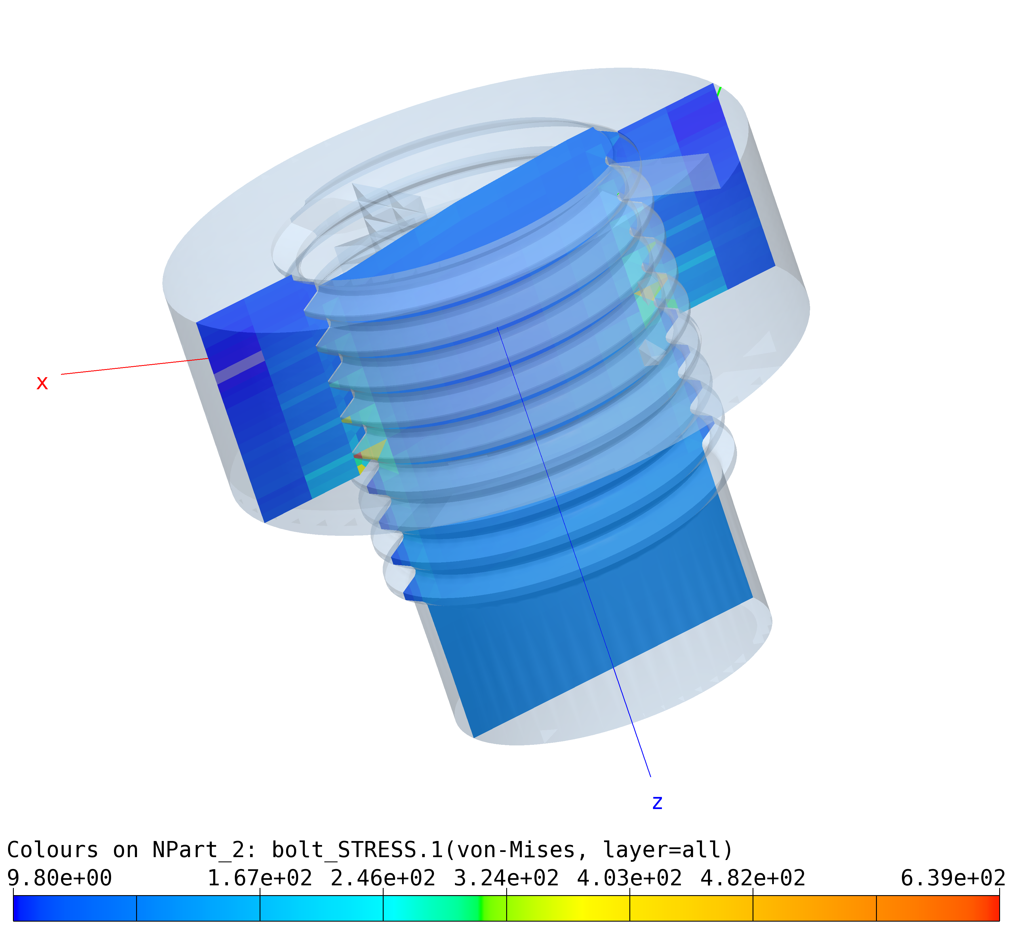
Bolt: Von Mises comparison stress on a cut through the semi-transparent solid mesh.
2.1.2. Cantilever Bracket
Note
Location of verification case:
verification/solid_mechanics/static/cantilever_bracket
One of K. J. Bathes incompressible material tests.
Cantilever bracket: Initial coarse mesh.
Cantilever bracket: Fines mesh.
Cantilever bracket: Solution with Q9.S.2D.UP3 elements. S1: Largest principal stress.
2.1.3. Cook Membrane Problem
Note
Location of verification case:
verification/solid_mechanics/static/cook_membrane
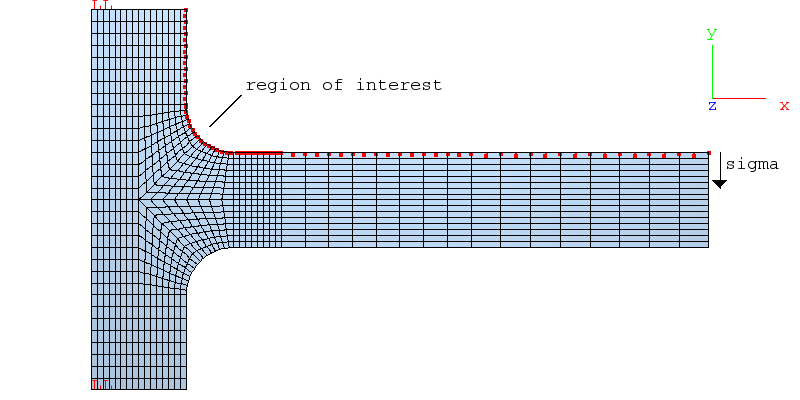
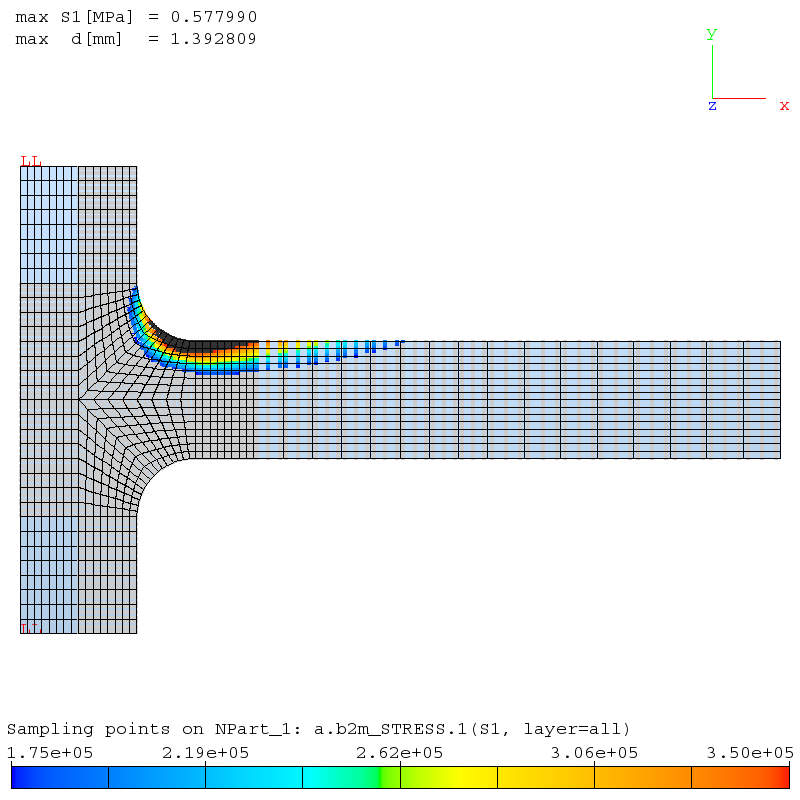
The Cook membrane problem is a classical test case for linear static analysis named after the author, R. D. Cook [cook1974] who first reported it. The structure consist of a trapezoidal surface in the x-y plane (see figure below and MDL input file for dimensions and material constants).
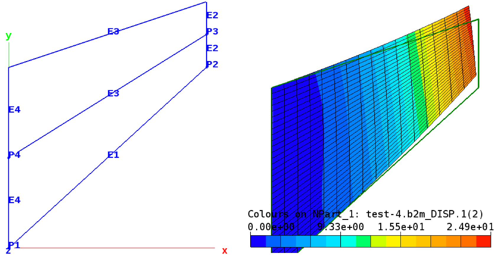
Mesh outlines (left) and initial mesh outline (green) and deformed FE mesh (right).
The structure is clamped along the edges E4 and it is loaded by a edge traction load along the edges E2 with a total load of 1 in the y direction.
The test is run with Q4.S.MITC.E4, Q8.S.MITC, Q9.S.MITC, and T3.S.MITC shell elements, comparing the global y-displacement at point P3 to the reported solution of 23.91:
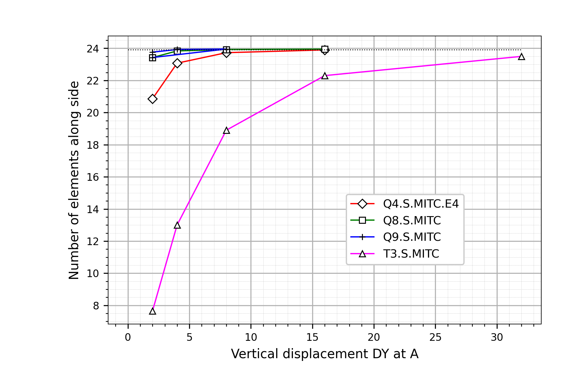
Cook membrane problem: Convergence behavior.
2.1.4. Deployable Ring
Note
Location of verification case:
verification/solid_mechanics/static/deployable_ring
The deployable ring problem was proposed by Goto et al. [goto] and it has been studied, among others, by Rebel [rebel], although with shell elements. It possesses the remarkable property that the ring can considerably be reduced in size by twisting it. The accompanying finite rotations in space make the deployable ring a severe test for the finite rotations capabilities of non-linear beam and shell elements.
The ring has a radius R = 60 and a rectangular cross section shape with a width of 0.6 a height of 6.0 and a modulus of elasticity of 2.0 105 [no units indicated]. It is clamped in one point and a rotation in the radial direction of the point opposite to the clamped point is applied. The rotation ranges from 0 to 2:math:pi.
The test is performed with B2 and B3 elements, the B3 elements obviously giving more accurate results because they approximate the circle better than the B2 elements. The FE mesh consist of a variable number of B2.S.RS or B3.S.RS elements. The figures below display the geometry and mesh points as well as results for a mesh with 36 B2.S.RS elements.
The analysis results with 36 B2.S.RS elements are displayed in the two figures below. The graph displays the applied moment:math:M_xx due to the applied rotation in the global x-direction, i.e the reaction to the applied rotation, as a function of the applied rotation.
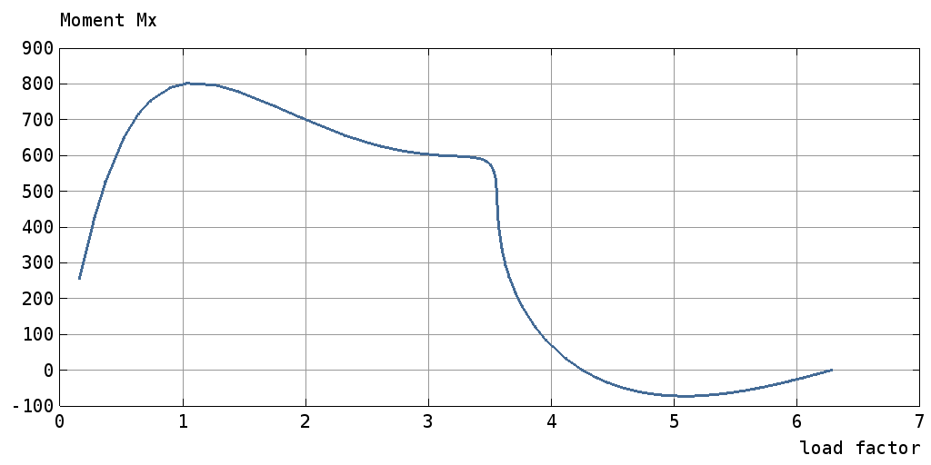
Deployable ring modeled with 36 B2.S.RS elements: \(M_xx\) vs applied rotation (36 B2.S.RS elements).
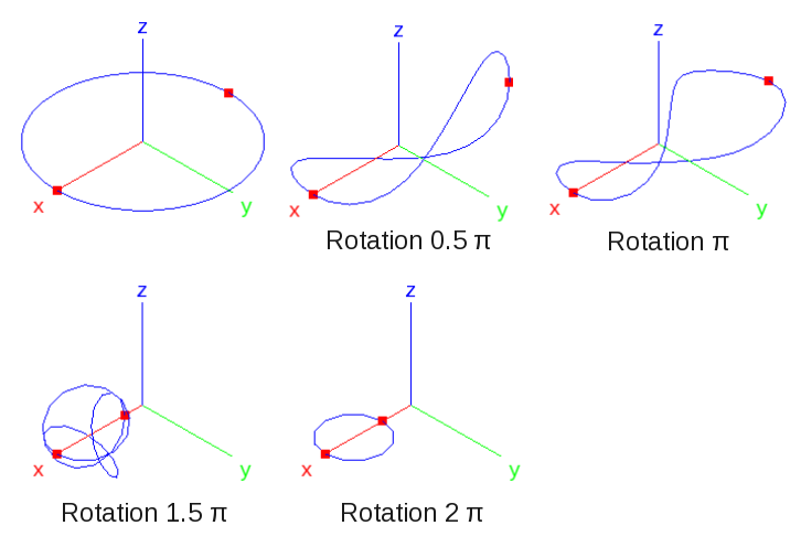
Deployable ring modeled with 36 B2.S.RS elements: Deformation shapes at steps 0:math:pi, 0.5:math:pi, \(pi\), 1.5:math:pi, and 2:math:pi. (36 B2.S.RS elements).
2.1.5. Hyperboloid Shell
Note
Location of verification case:
verification/solid_mechanics/static/hyperboloid_shell
A hyperboloid shell model is generated with 3 and 6 node triangular elements for several mesh densities, testing the convergence. The test compares to results from
Do-Nyun, Klaus-Jurgen Bathe; A Triangular six-node shell element; Computers and Structures, Volume 87 Issue 23-24, December, 2009, Pages 1451-1460.
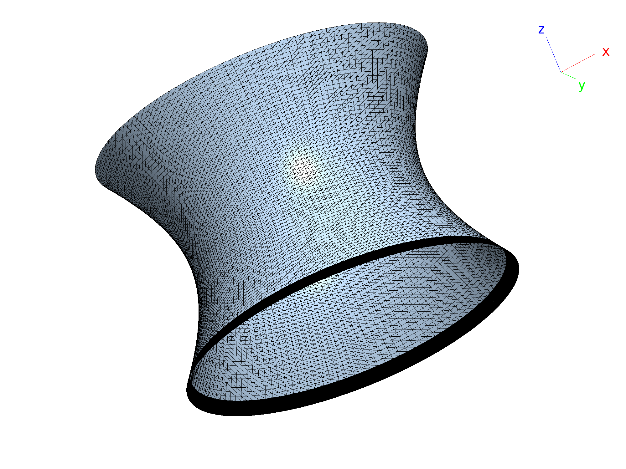
Hyperboloid shell test: Triangular mesh (TR3 elements) with highest mesh density of test.
A particularity of this test is the generation of the hyperboloid shell: B2000++ epatch meshes cannot generate hyperboloid surfaces. Therefore, a cylinder is generated and the nodes changed after the initial b2ip++ run, see__init__.py.
2.1.6. Lee’s Frame Problem
Note
Location of verification case:
verification/solid_mechanics/static/lee_frame
Lee’s frame is a simple frame structure subject to large displacements
and rotations. The B2000++ model defined in file frame.mdl follows
the original geometry and loading, and it is clamped at both ends.
Analysis is performed by means of the B2.S.RS Reissner-Simo beam
element. The test also checks the beam local coordinate system
orientation option (defined by a reference node or by a reference
orientation vector).
Lee frame: Beam model and load (dense mesh).
Two tests are executed, one with applying a force as shown in the
above picture, and another with a ‘displacement loading’
instead. Solver options (see case command in input file) for the
force case are
analysis               nonlinear
increment_control_type hyperplane
step_size_max          10 # To get a curve with some points...
ebc                    1 # zero constraints set
nbc                    1 # applied force set
join                   0 # Needed because more than one epatch
The structure deforms until it reaches an unstable state, after which a new stable state is reached. Using the continuation processor, the complete static solution can be obtained as displayed in the load-displacement plot below.
Lee frame: Load-displacement response point A (continuation).
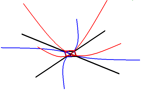
2.1.7. Node Section Forces
Location of case: $B2VERIFICATION/solid_mechanics/static/node_section_forces
This test demonstrates and checks the extraction of beam and rod element section forces of selected elements attached to a node. Element section forces must be extracted when reaction forces at the border of mesh parts are required, such as hinges.
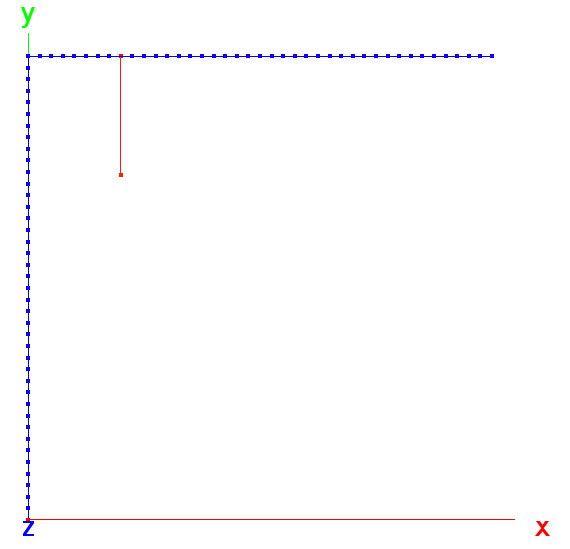
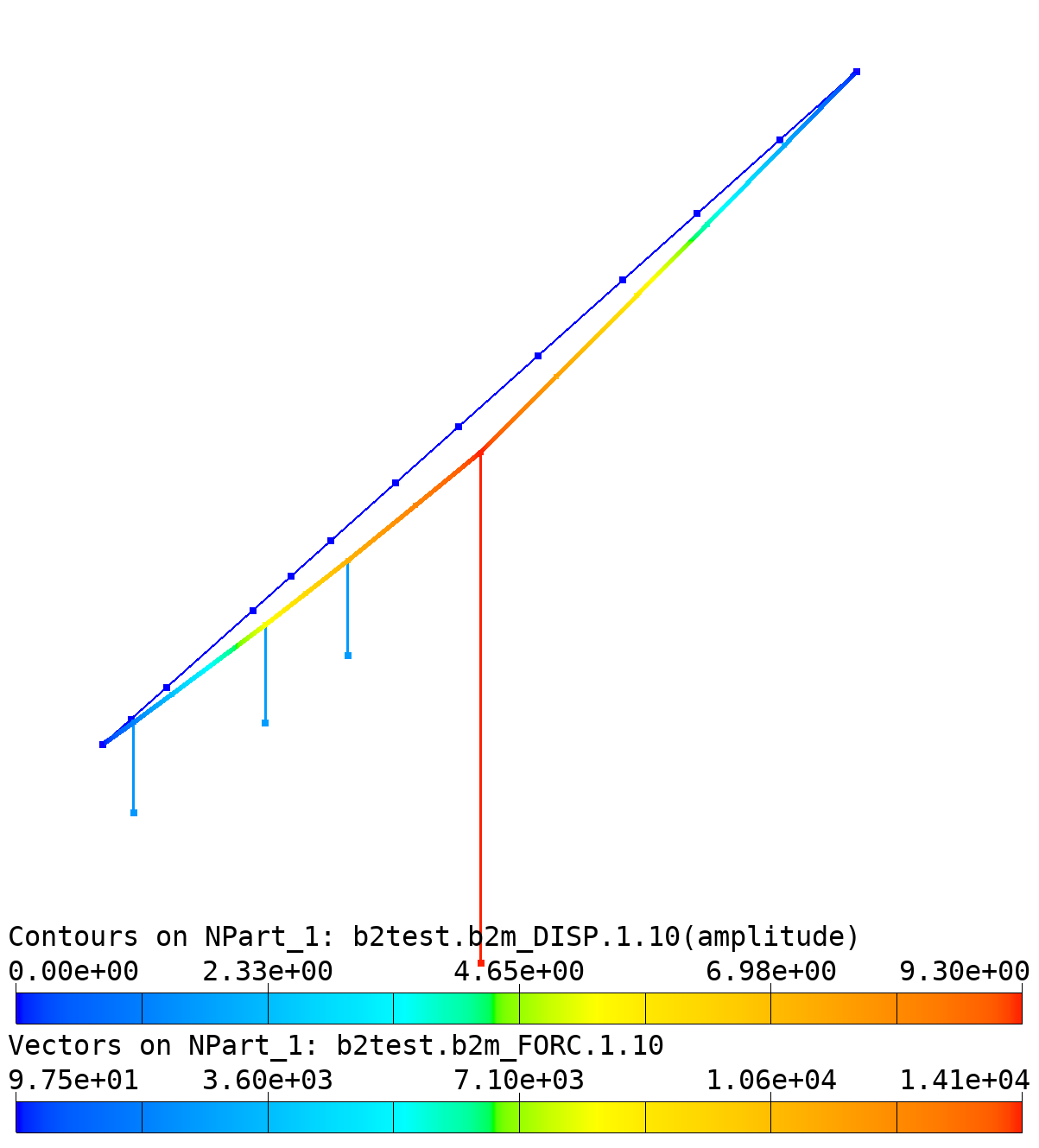
Tests are made with rods and beams, checking the element-local to global force (and moment) transformations). The model is a simple truss clamped at x=0 and loaded by a concentrated force (see figure below).
The model is generated with MDL files and a linear analysis is
performed with B2000++. Thereafter the Simples post-processing scripts
rods.py and beams.py loop over a list of tuples (nodeid,
elemid1, elemid2, ...) where nodeid is the node identifier to
which elements are attached and the elemid are the rod or cable
element identifiers attached to that node. For each tuple (nodeid,
elemid1, elemid2, ...) the script loops over the elements and
extracts section forces and moments (if any) of each element
elemidat the nodenodeid,transforms the forces and moments to the global coordinate system,
Sums up the resulting forces (and moments) at the node.
In this particular test case the sum of the element forces must be equal to the reaction forces, because the nodes are the constrained nodes.

Red: Deformed mesh (amplified). Blue: Mesh.
The test script rods.py launches the rod test case and is
listed below:
"""Simples script to extract rod forces of selected elements attached
to a node and to sum them up.
"""

import os
import sys

import numpy
import simples as si

numpy.set_printoptions(precision=1)

if os.system('b2000++ rods.mdl'):
    sys.exit(1)

verbose = 0
if len(sys.argv) > 1:
    verbose = int(sys.argv[1])  # Set to 1 for result output

m = si.Model('rods.b2m')
Branch = m.get_branch(1)

#Extract rod forces (axial forces)
rforces = si.SamplingPointField(m, 'FORCE_ELEMENT', case=1)

Ftot = numpy.zeros(3) # Total force on structure (for equilibrium
                      # check only)

# Loop over all lists (nodeid, elemid1, elemid2, ...)
for elist in ((1,1,2), (4,3)):
    F = numpy.zeros(3) # Sum of forces of selected elements
    for eid in elist[1:]:
        e = Branch.get_elem(eid)
        forcev = numpy.array([rforces[eid][0,0], 0., 0.]) # Local force vector
        f = numpy.dot(forcev, e.elbase) # Transform to global
        if verbose == 2:
            print(e.elbase)
        F += f
    if verbose == 1:
        print(f'Node {elist[0]}: Section forces sum F={F}')
    Ftot += F
if verbose == 1:
    print(f'Ftot={Ftot}')
if not numpy.allclose(Ftot, numpy.array((0, -1000, 0))):
    print(f'***ERRIOR: No equilibrium, Ftot={Ftot}, required=[0,1000,0]')
    sys.exit(1)
2.1.8. Raasch Challenge Test
Note
Location of verification case:
verification/solid_mechanics/static/raasch_challenge
The Raasch challenge test is a linear shell test case where drill rotations, i.e shell in-plane rotations, play an essential role. The problem has been presented by Knight [knight1997]. The geometry has the form of a clamped ‘hook’, i.e. a thick curved strip with a small radius followed by an arc with a larger radius. The model was used by G. Rebel in his PhD thesis [rebel] to demonstrate the performance of his shell elements in B2000++ However, in the example the MITC shell elements are used.
The FE model consist of two cylindrical patches, both with a length of
20. The first patch has a radius of 46 and spanning an angle of
150 degrees. The second smaller patch has a radius of 14 and spanning
an angle of 60 degrees in the other direction. The mesh can be
parameterized (see the MDL input file raasch.mdl). Note that, in
contrast to previous versions of this model, both cylindrical mesh
patches are placed in the default branch 1.
is not specified anymore.

Raasch challenge: Model.
The analysis is performed with 4, 8, and 9 node MITC shell elements.
Note that the B2000++ MITC shell elements are 5/6 dof’s per node
elements. To avoid singularities with in-plane rotations, B2000++
automatically defines the correct node types: Nodes with constraints
(EBC conditions) and nodes where elements at a given limit angle meet
will become 6 DOF nodes, while all other nodes are 5 DOF nodes or
nodes of another type. The solution (deformed shape and von Mises
stress) for the Q4.S.MITC.E4 elements and a fine grid, with the
initial shape plotted with outline only, is shown below.
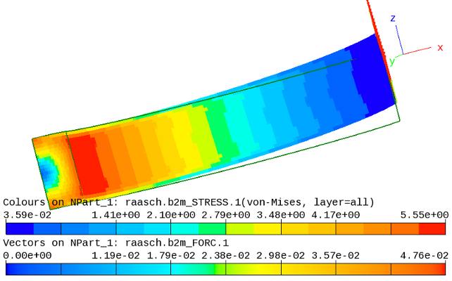
Raasch challenge: Deformed structure (amplified x 4).
The reference solution by Knight for the tip displacement in z direction is 4.9352. Reference solutions for stresses are not given.
2.1.9. Tensile Strip with Hole
Note
Location of verification case:
verification/solid_mechanics/static/strip_with_circular_hole
Stresses and the stress intensity factor in a aluminum tensile strip with a circular hole are computed with solid elements. The test originates from a mesh generated at CIRA s.p.a. for 2- and 3-dimensional solid analysis.
The strip with circular hole is described in section Tensile Strip with Hole of the Simples documentation.
2.1.10. Tower Cable
Note
Location of verification case:
verification/solid_mechanics/static/tower_cable
An initially straight cable is loaded by point masses, the cable’s own weight, and point masses. The static equilibrium and the eigenfrequencies around the static equilibrium are computed. This test originates from an older ADINA test case description [bathe1976] and has been converted to the MKS system of units.
Tower Cable: Mesh, deformed shape, and forces (due tu mass acceleration).
The cable is prestressed with an initial stress, initial strain, or
initial force (see input file cable.mdl). All 3 variants are
tested, checking the final deformed position and the cable forces. The
dead weights are introduced by means of point masses and referenced in
the natural boundary condition case nbc 1 (file cable.mdl)
with the terrestrial gravitational acceleration in the proper
direction, i.e. the negative y-axis. Note that the vibration analysis
case (case 2) may not reference the natural boundary condition case
nbc 1, because it would re-introduce the boundary condition a
second time.
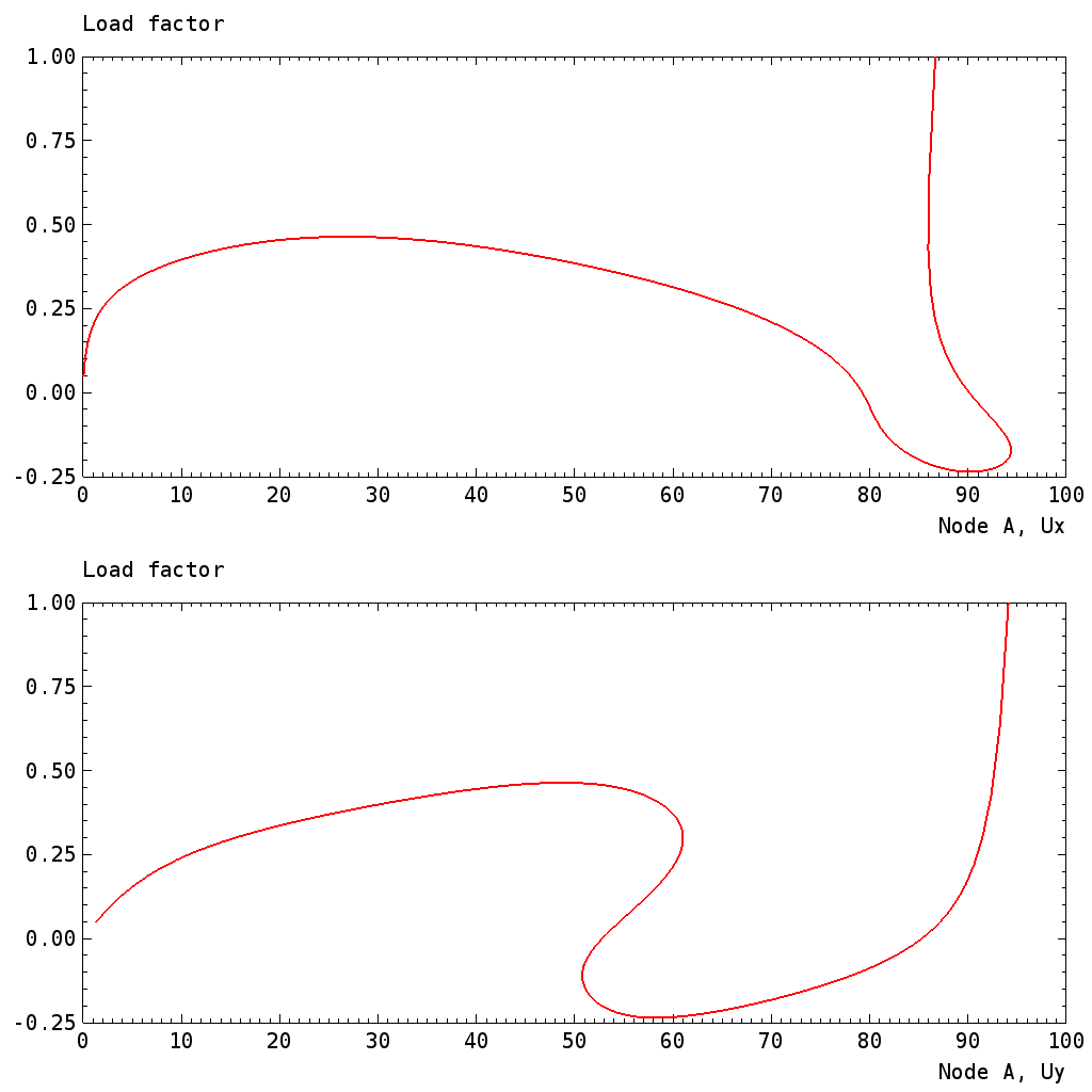
The static load-displacement response of a node (node A) and the deformed configuration are shown in the figures below. Values correspond to those of the ADINA test case description.

Tower Cable: Load-displacement and load-stress curves of node A (values in [in]).
The vibration analysis with prestress results (the equilibrium
position for the load factor 1.0) are listed in the table below. To
perform a restart with a given equilibrium solution the dof_init
option has to be added to the case defining the free vibration analysis
(here: case 2)
case 2
   ...
   dof_init 'DISP.*.10.0.1'
   ...
end
or in the command line to B2000++
prompt> b2000++ -adir dof_init=DISP.*.10.0.1 -adir case=2 DBNAME
The first eigenfrequency \(f_1=0.226 Hz\) computed by B2000+++ is identical, to 3 decimal places, to the solution reported in [bathe1976].
A Simples script :file:run.py computes eigenfrequencies as a
function of the load factor:
"""Compute eigenfrequencies as a function of the load factor
"""

import os
import numpy
import simples as si
from simples import constants as const

def fixmodecycle(db, case, cycle):
    # Renames the MODE datsets: B2000++ save the MODE datasets with
    # cycle 0 irrespective of the actual cycle for which K is computed!
    sets = sorted(db.keys(f'MODE.1.0.0.{case}.*'))
    for s in sets:
        newname = f"MODE.1.{cycle}.0.{case}.{s.split('.')[5]}"
        db[s].name = newname

# Solve nonlinear problem.
os.system("b2000++ -define init=2 -adir cases=1 cable.mdl")

# Get computed steps
m = si.Model('cable.b2m')
steps = m.get_steps(case=1)
m.close()

x = []
y = []
for c, loadfactor in enumerate(steps):
    cycle = c + 1
    print(f"Compute eigenmodes for loadfactor {loadfactor}")
    os.system(f"b2000++ -adir cases=2 -adir dof_init='DISP.*.{cycle}.0.1' cable.b2m")
    m = si.Model('cable.b2m')
    fixmodecycle(m.get_db(), 2, cycle)
    result = m.get_eigenfrequencies(case=2, cycle=cycle)
    x.append(loadfactor)
    y.append(result.frequency)
    m.close()

# Create a graph
g = si.Graph2()
g.axes_label_x = 'Load factor'
g.axes_label_y = 'Eigenfrequency [Hz]'

# Add lines
for mode, color in zip((1,2,3), ("RED1", "GREEN1", "BLUE1")):
    v = []
    for yy in y:
        v.append(yy[mode-1])
    line = g.add_line(x, v, label=f'Mode {mode}')
    line.marker = 'o'
    line.color = const.RGBCOLORS[color]

g.add_legend()
g.axes_minmax_x = (0., 1.)
g.save('output.svg')
print('Created plot file output.svg')

Tower Cable: Eigenfrequencies of first 3 modes as a function of load factor.
2.2. Buckling Analysis
2.2.1. Slit Open Annular Plate
Note
Location of verification case:
verification/solid_mechanics/buckling/annular_plate
This test case was proposed by Basar and Ding [basar1992] and is also reported by Buechter and Ramm [buechter1992] and by Rebel [rebel]. It features an annular plate in the xy-plane with a slit, with one side of the slit clamped and the other side subject to a line load p in the z-direction.

Slit Open Annular Plate: Test case definition
A nonlinear analysis is performed with the following case definition:
case 1
  analysis              nonlinear
  ebc                   1
  nbc                   1
  max_newton_iterations 50
  newton_method         conventional
  max_step              500
  step_size_min         0.001
  step_size_init        0.01
end
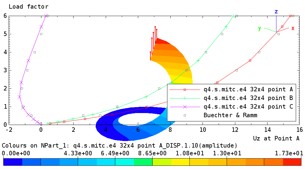
The figure below displays the z-displacements at points A, B, and C plotted against the applied load for a 32x4 mesh of Q4.S.MITC.E4 elements and the final deformed configuration at the maximum load factor_6.
2.2.2. Collapse Analysis of Cylindrical Arch
Folder: $B2VERIFICATION/solid_mechanics/buckling/arch_14
A cylindrical arch clamped on both ends is subject to a mid-span point load compressing the arch. The structure is modeled by beam and shell elements.
Cylindrical arch: Beam mesh and applied load.
This structure exhibits a typical snap-through behavior, see the plot of the mid-span y-displacement vs load factor and the plot of the final deformation:

Cylindrical arch: Final deformation, load factor 1.
2.2.3. Linear Buckling of Box Beam
Note
Location of verification case:
verification/solid_mechanics/buckling/box_beam
The linear buckling load of a slender beam subject to axial compression is computed. The beam is clamped on both ends and its section consists of a thin-walled box symmetric with respect to the cross section y- and z-axes. Buckling is triggered either by an imposed axial displacement or a force in the axial direction.
Both a beam mesh and a shell mesh are tested:
Beam mesh 1: Linear B2.S.RS elements with boundary conditions imposed on both beam end nodes and section properties imposed by beam properties.
Beam mesh 2: Linear B2.S.RS elements with boundary conditions imposed on both beam end nodes and section properties imposed by a beam section sub-model.
The shell mesh consists of element patches of Q elements forming the box. To impose correct boundary conditions for the shell model, i.e. to prevent the end sections from deforming, RBE-type constraints have to be imposed on either beam end, defining the boundary conditions on the reference nodes 100000 and 100001:

Shell model: RBE constraints on either beam end.
The theoretical solution (Euler formula) is readily obtained from the literature:
where \(E\) is the modulus of elasticity, \(J\) the moment of inertia, and \(L\) the length of the clamped beam. With \(E=70 GPa\), \(L=1.0 m\), box width and height \(W=0.02 m\), wall thickness \(t=0.001m\), the critical load is \(P_{cr}= 12671N\).
Shell model: First buckling mode, both beam ends clamped.
2.2.4. Channel Section Beam Problem
Note
Location of verification case:
verification/solid_mechanics/buckling/channel_section_beam
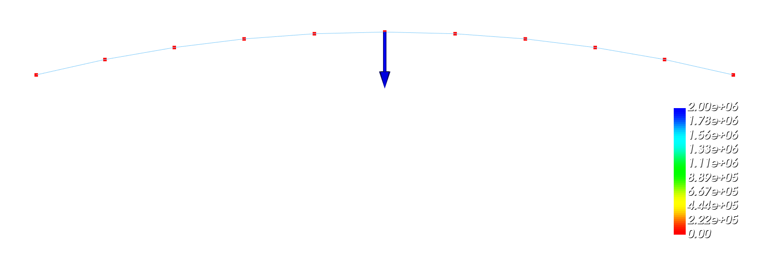
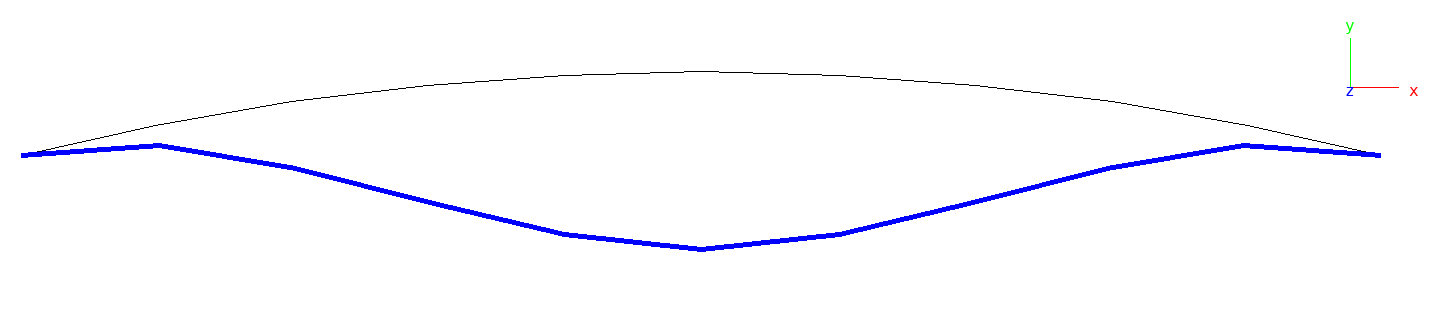
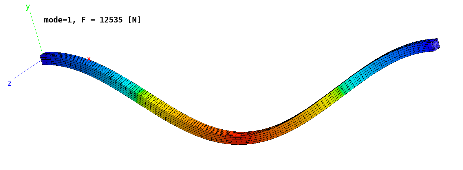
A clamped beam with a C-section (‘channel section beam’) described by Betsch et al. [2] is subject to displacement constraints in the global y-direction. The beam is modeled with Q4, Q8, and Q9 shell elements. Results are displayed below for the Q4, Q8, and Q9 meshes.

Buckling of channel section beam: Q4 mesh solution.
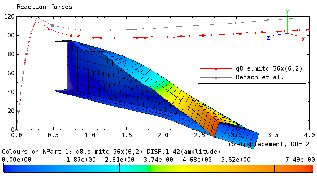
Buckling of channel section beam: Q8 mesh solution.

Buckling of channel section beam: Q9 mesh solution.
2.2.5. Curved Panel
Folder: $B2VERIFICATION/solid_mechanics/buckling/cylinder_cutout
The test case computes the post-buckling behavior of a slightly curved panel, comparing results with different shell element types.
The panel has a length L=92mm along the straight edges, a radius R=586mm with an angle \(\alpha\) of 9 degrees along the curved edges and a thickness t=1mm. The mesh grid is 7 by 7 nodes in both directions. Due to symmetry only one quarter of the panel is considered.

Buckling of slightly curved cylindrical panel: Geometry
The material is linear isotropic, with modulus of elasticity E=7*104N/mm2 and poisson=0.3.
Line loads are applied on edge I in the positive z direction. Edge I has suppressed displacements in radial direction and edge IV is simply supported. Edges II and III have symmetry boundary conditions.
No analytical solutions are available for this problem. The results of
the analysis, i.e the buckling load values, can be consulted in the test
file __init__.py. The figure below display the convergence behaviour
of this problem.
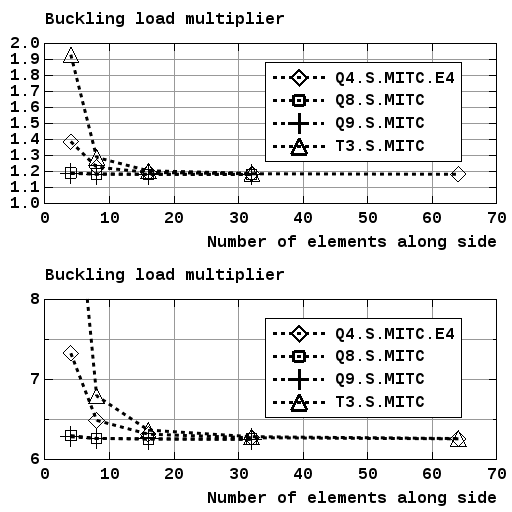
Buckling of slightly curved panel: Convergence behaviour (force controlled)
2.2.6. Cylinder under Torsion Load
Note
Location of verification case:
verification/buckling/cylinder_torsion
The torsion buckling load of a cylinder is computed. The cylinder is
clamped on one end and subject to a torsional load on the other free
end. Dimensions of the cylinder as defined by the epatch command
of the MDL input file:
length 4000
radius 500
phi1 0 phi2 360
thickness 1
The material is linear isotropic (see input file), and the cylinder is meshed with 36 elements (Q4) or 18 elements (Q8/Q9) in circumferential direction and 20 elements (Q4) or 10 elements (Q8/Q9) in axial direction.
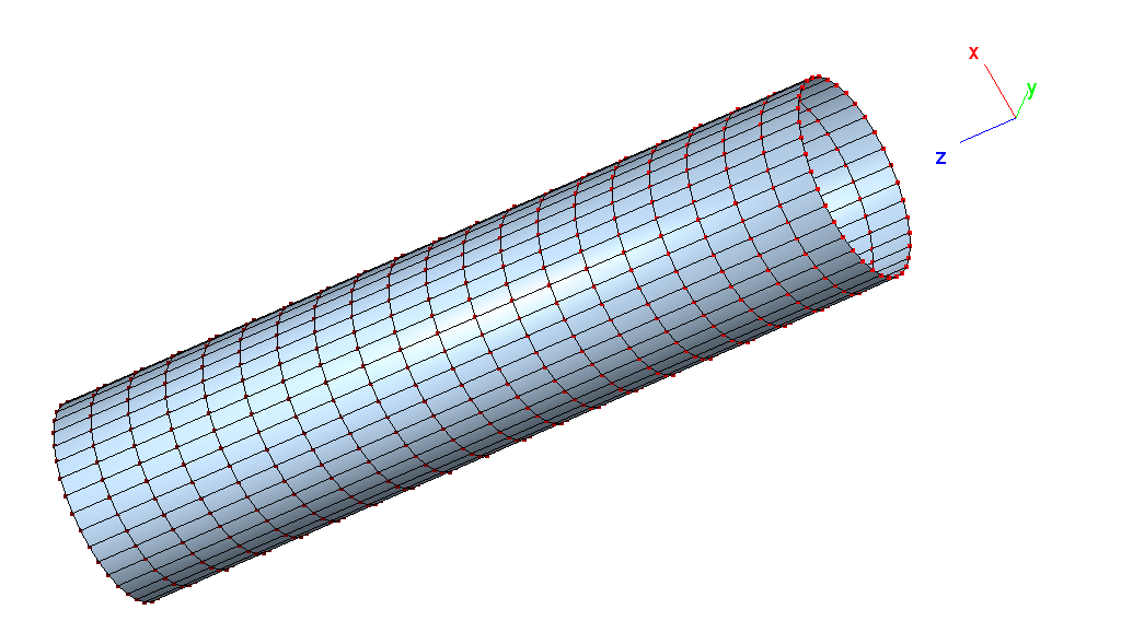
Cylinder under torsion load: Mesh (Q4 shell elements).
Note: The cylinder mesh generator of epatch does not automatically
close the cylinder if the angles are 0 and 360 respectively. This has
to be done by the user with the join command:
join 0
   automatic
end
Analysis is performed with the meshes described above and compared to a reference solution obtained with a fine Q4 mesh 288 by 144 elements. Results are displayed in the table below: While the Q4 and Q8 meshes deliver results with a 15% error with respect to the reference solution, the Q9 mesh performs very well.
Element type |
λ1 |
λ2 |
λ3 |
λ4 |
Q4.MITC.E4 ref. |
0.6004 |
0.6004 |
0.6277 |
0.6277 |
Q4.MITC.E4 |
0.709 |
0.709 |
0.727 |
0.727 |
Q8.S.MITC |
0.709 |
0.709 |
0.727 |
0.727 |
Q9.S.MITC |
0.6004 |
0.6004 |
0.6277 |
0.6277 |
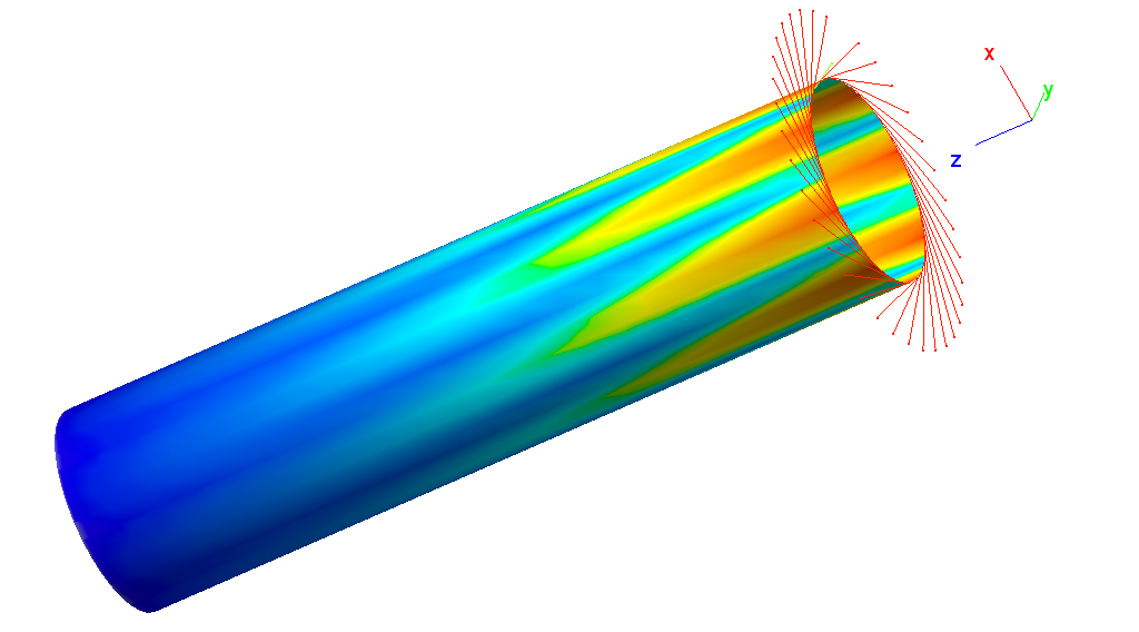
Cylinder under torsion load: First buckling mode and applied generated torsional forces (Q4 shell elements).
2.2.7. Hinged Cylindrical Shell
Note
Location of verification case:
verification/solid_mechanics/buckling/cylindrical_shell_hinged
A slightly curved cylindrical panel is loaded with a central concentrated out-ot-plane force. Computations are performed with Q4.S.MITC, Q4.S.MITC.E4, Q8.S.MITC, Q9.S.MITC,
Results from:
Ramm E.: ‘The Riks/Wempner approach - An extension of the displacement control method in nonlinear behavior of cylindrical shells’, Recent Advances in Non-linear Computational Mechanics, Chapter 3. Pineridge Press Limited: Swansea, U.K. , pp 63 - 86, 1982
Pedro et al.: , ‘A finite strain quadrilateral shell element based on discrete Kirchhoff-Love constraints’, International Journal for Numerical Methods in Engineering, Vol 64, 2005, pp 1166 - 1206
Mesh and essential boundary conditions.

Q4 mesh: Ux displacement as a function of the load factor, point A.

Q4 mesh: Ux displacement as a function of the load factor, point B.

All element types: Ux displacement as a function of the load factor, point A.

All element types: Ux displacement as a function of the load factor, point B.
2.2.8. Euler Buckling of Beam
Note
Location of verification case:
verification/solid_mechanics/buckling/euler
The test computes the buckling load of a clamped beam modeled by beam elements and subject to compression and to eccentric load application. This test corresponds to one of the classical Euler buckling problems and it illustrates the capability of the B2000++ environment of dealing with multiple parametric runs with a single input file.
The beam has a length of 1m and a cross section of 0.01m by 0.01m, the
cross section being described by a MDL property command of type
rectangle:
property 100
    beam_section
    mid 1
    shape rectangle
    d1 0.01 # width
    d2 0.01 # height
end
The material is a standard isotropic material (steel) described by a MDL
material command of type isotropic:
material 1 isotropic
  e 210.0e9
  nu 0.3
end
The beam is modeled by a MDL epatch command with 2 node beams:
epatch 1
  geometry line
  p1 0 0 0
  p2 1.0 0 0
  eltype B2.S.RS
  beam_offsets 0. (EY) (EZ) 0. (EY) (EZ)
  beam_orientation 0 1 0
  ne1 (NE)
  pid 100
end
The beam offsets are parameterized (beam_offset option): For each run
the EY, EZ, and NE parameters will have to be passed to
B2000++. Several runs with different parameters, together with the
extraction of the buckling load, will define the diagram below.
The analytic solution (Euler buckling) is readily obtained from the
literature, see run.py script.
The test loop computes the decrease of the buckling load when an eccentric compression force is applied. Each test is executed with the one of the Python utilities, which allows for passing parameters to the input file:
xy=[]
t = 0.01 # Nominal eccentricity (=beam section width)
print('{:10s} {:10s}'.format('Ecc. ratio', 'Pcr/Pcr0'))
for ez in (0., t/100., t/75., t/50., t/25., t/10., t/7.5, t/5., t/2.5, t):
    # Run B2000++ with current parameters passed to B2000++
    os.system('rm -rf beam.b2m')
    if si.util.solve('beam.mdl', params={'EY': 0.0, 'EZ': ez}):
        model = si.Model('beam')
        result = model.get_buckling_load()
        model.close()
        pcr = result.bloads[0]
        if ez == 0.0:
            # Pcrit without eccentricity
            pcr0 = pcr
        # Append to tuple
        xy.append((ez/t, pcr/pcr0))
        print('{:10.5f} {:10.5f}'.format(ez/t, pcr/pcr0))
    else:
        print('Run failed for e/t=', ez/t)
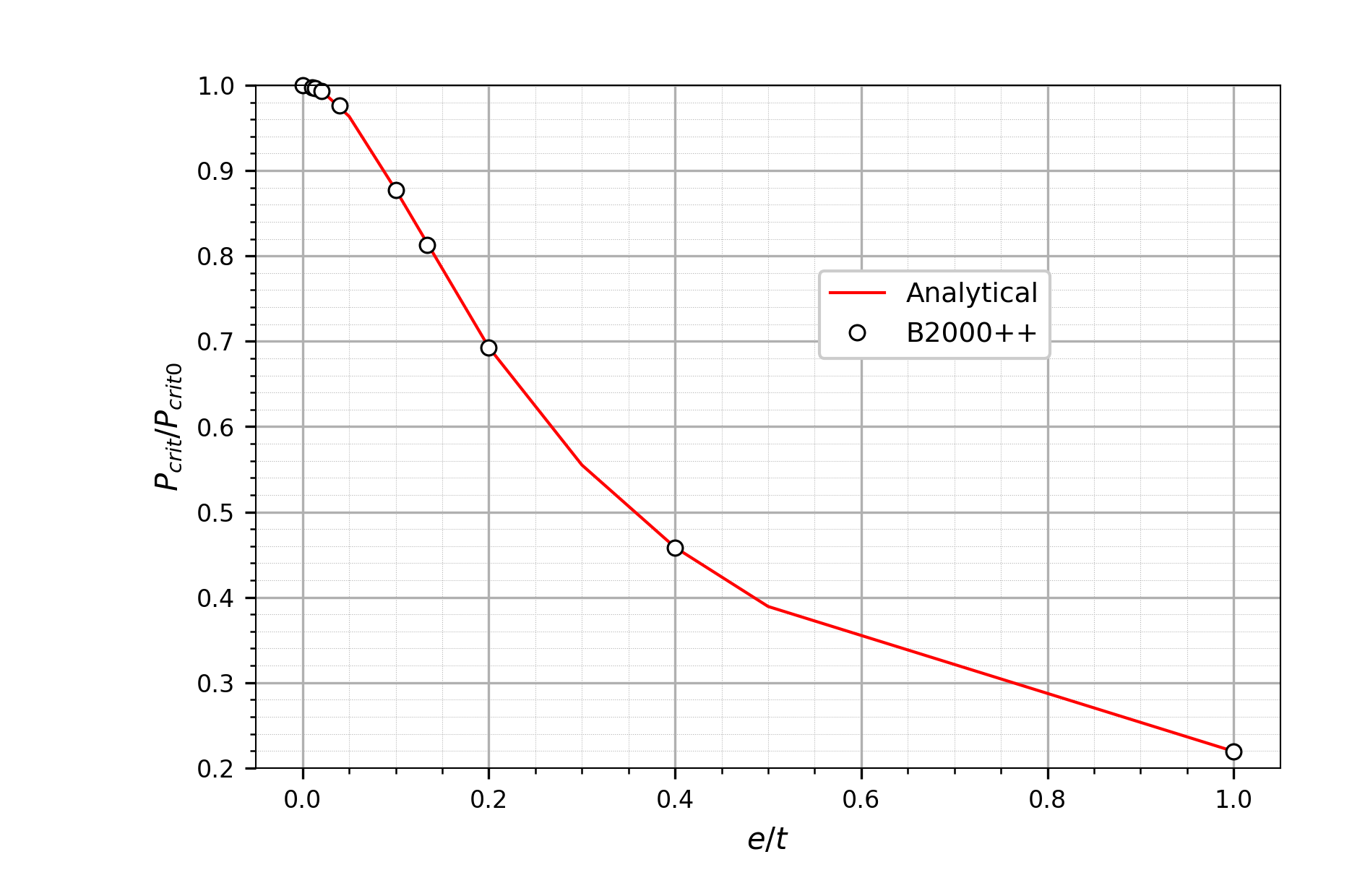
Reduction of buckling load as a function of beam section eccentricity ratio eccentricity/thickness for B2.S.RS (2 node beam) elements.
2.2.9. L-Shaped Frame
Note
Location of verification case:
verification/solid_mechanics/buckling/frame_clamped
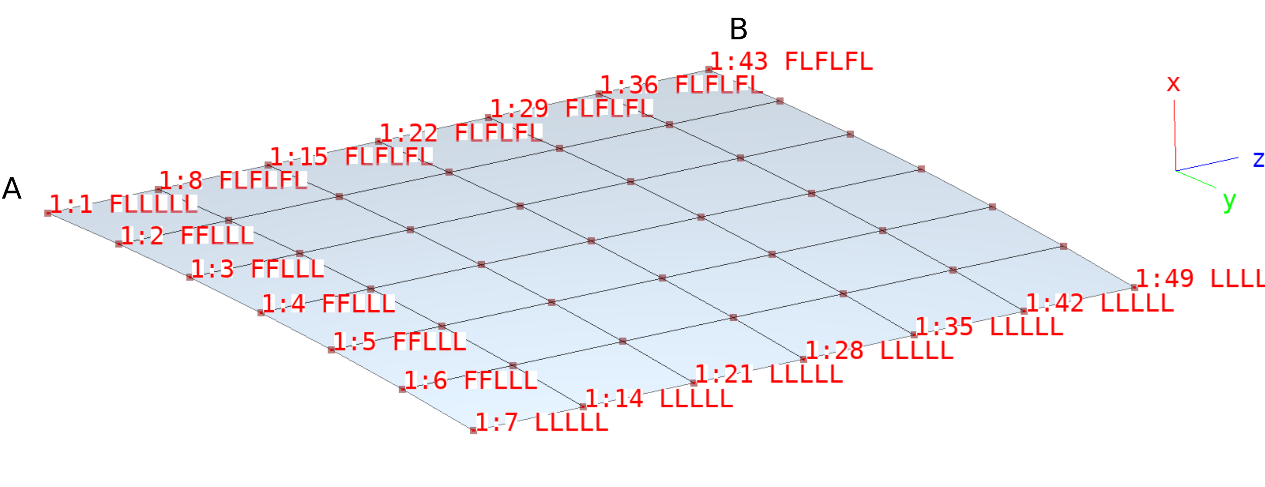
An L-shape frame is modeled in the x-y plane with shell elements. It is clamped on one end and loaded at the other end at (0,0,0) by a force \(F_y\), see figure below. To trigger buckling a small force in the z direction is applied at (0,0,0).
This problem has been reported, among others, by Nour-Omid and Rankin [3].

Buckling of L-shaped frame: FE mesh and boundary conditions. Force Fz at point A (0,0,0) not shown.
To get beyond the buckling load the “hyperplane” increment control
strategy has been selected, see input file b2test.mdl. The
diagram and the deformed shape plot below illustrate the nonlinear
behavior:

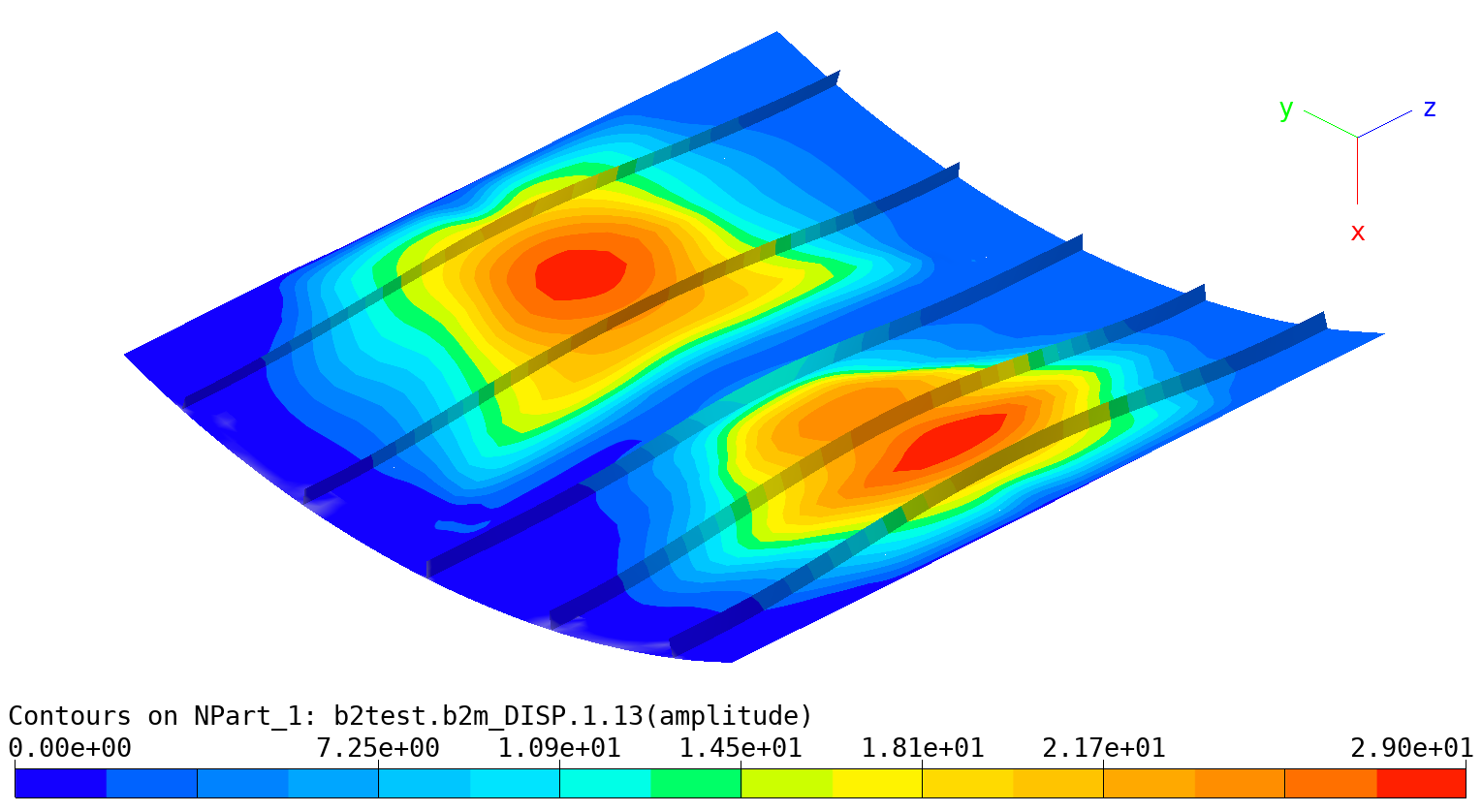
Buckling of L-shaped frame: Out-of plane displacement DZ at point A (0,0,0) vs applied force Fz at point A.
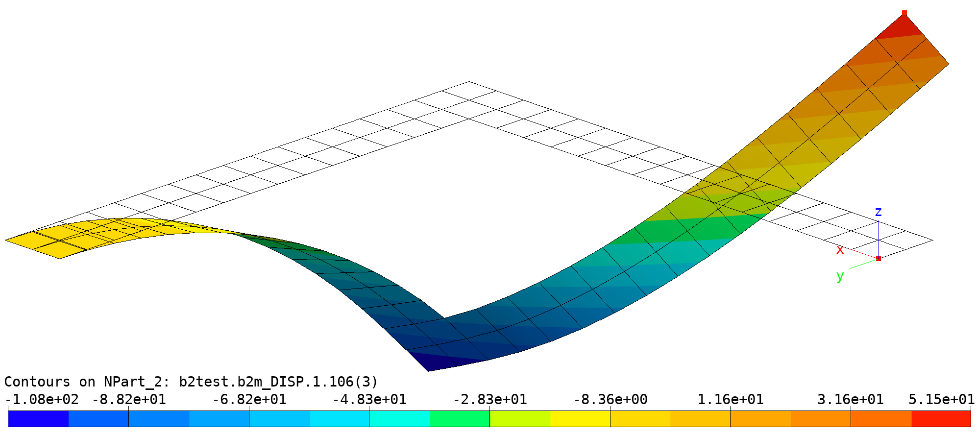
Buckling of L-shaped frame: Final deformed state and undeformed mesh.
2.2.10. Hexadome
Note
Location of verification case:
verification/solid_mechanics/buckling/healey_hexadome
This test checks the performance of rod elements in the post-buckling range. It consists of a shallow truss structure referred to as a hexadome. The hexadome was first analyzed by Tim Healey [healey]. The rods have a length L=9m, with the height h=1.5m and the rod cross section area A=1cm2. At each of the intersection nodes (where more than two bars are attached to a node), an external force F=10N is applied. The structure is simply supported. Every bar in the structure is modeled with one rod element.
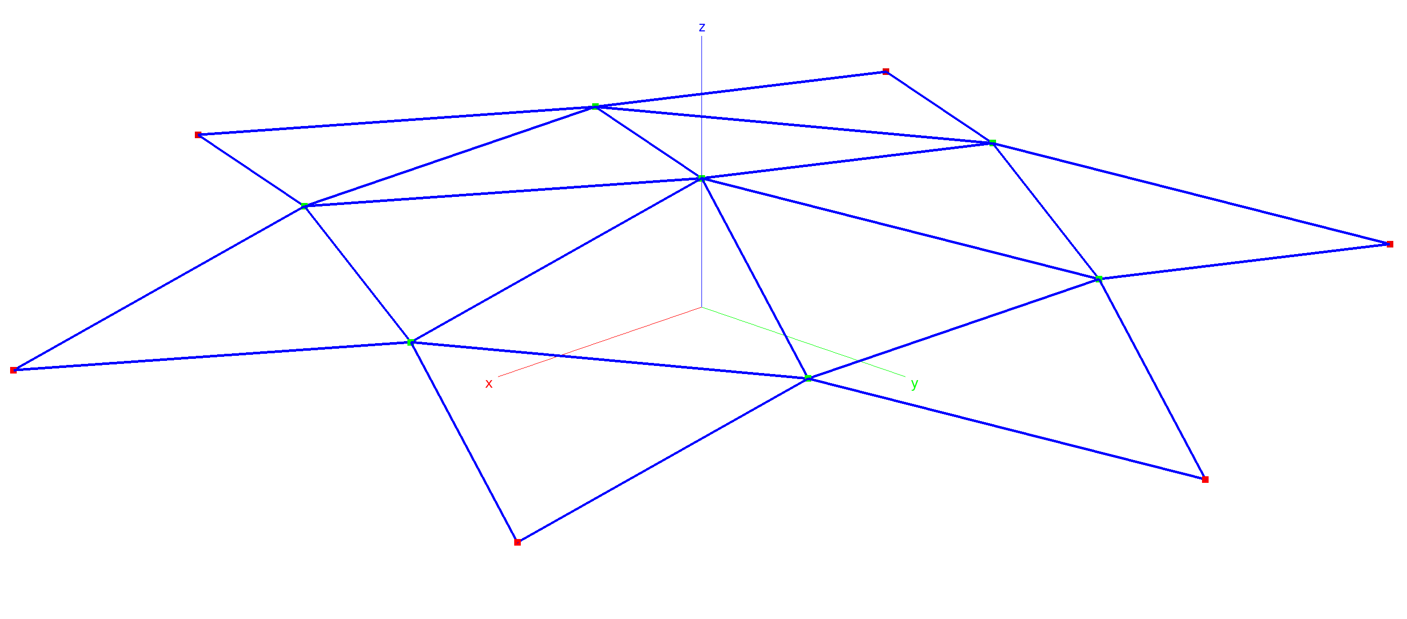
Healey dome geometry. Green dots: Free nodes loaded in z-direction. Red dots: Locked nodes.
The nodes of the rod elements have three translational degrees of
freedom. For this reason the rod elements can only be simply
supported, the bending stiffness of a rod element being zero. The dome
only buckles as a result of the instability of the construction, not
as a result of the local buckling of a single bar! Due to the forces,
the rods shorten, and at a certain point the dome becomes unstable and
it buckles. Since rods have only stiffness in axial direction only one
element can be used to model a bar over the length L. The material is
linear isotropic, see input file b2test.mdl.
x
The results displayed below were obtained with increment control type
hyperplane. To make sure that the whole path is captured, an
initial load factor increment of 0.01, a maximum step size of 0.2 were
selected, up to a final load factor of 5.0. The load factor increases
and decreases several times during the buckling process, as shown in
the load-displacement curve for the mid-point node below.

Load-displacement curve of mid-point node
The test checks the final displacement state for a load fact or of 5.0. Intermediate steps are not checked.
2.2.11. Cylindrical Panel (PSC5)
This composite stiffened panel, originating from a Nastran BDF file, is one of the COCOMAT [cocomat] benchmark problems (see [ha1], [ha2], [ha3]). It has the particularity that the shell elements of the stringer feet require an offset with respect to the neutral axis. This can be modeled with B2000++ in two ways
Using ‘air layers’: The air layers are taken into account the calculation of the total volume of the model, resulting in a difference of volume between the two models.
Defining an eccentricity for specific elements.
The panel mesh and boundary conditions, as generated from the converted Nastran BDF file, are visualized with baspl++:
COCOMAT panel: FE mesh and boundary conditions.
The linear buckling analysis (case 1) calculates the 10 lowest buckling loads:
b2000++ -define case=1 psc5.mdl
Display the buckling loads with the b2print_buckling_loads app:
b2print_buckling_loads --case=1 psc5.b2m

Eigenvalues and buckling loads, case=1, cycle=0

     MODENUM       LAMBDA        PCRIT
           1       0.6268   74255.8861
           2       0.7199   85284.2718
           3       0.7573   89715.7311
           4       0.7700   91221.8463
           5       0.7964   94348.4640
           6       0.8020   95010.2810
           7       0.8079   95710.3395
           8       0.8168   96769.3425
           9       0.8257   97823.4730
          10       0.8335   98743.5306

Contributing EBC identifiers: 3
Total reaction force Ftot=(-2070, -34.56, -1.185e+05)
Force amplitude=1.185e+05
LAMBDA (eigenvalue): if > 1 no buckling, < 1 buckling, marked by *
PCRIT (critical load): F * LAMBDA (if F != 0)
Reaction force: Sum of reactions due to EBC and NBC
A comparison of the lowest eigenmode with an simulation performed with Abaqus 6.4:
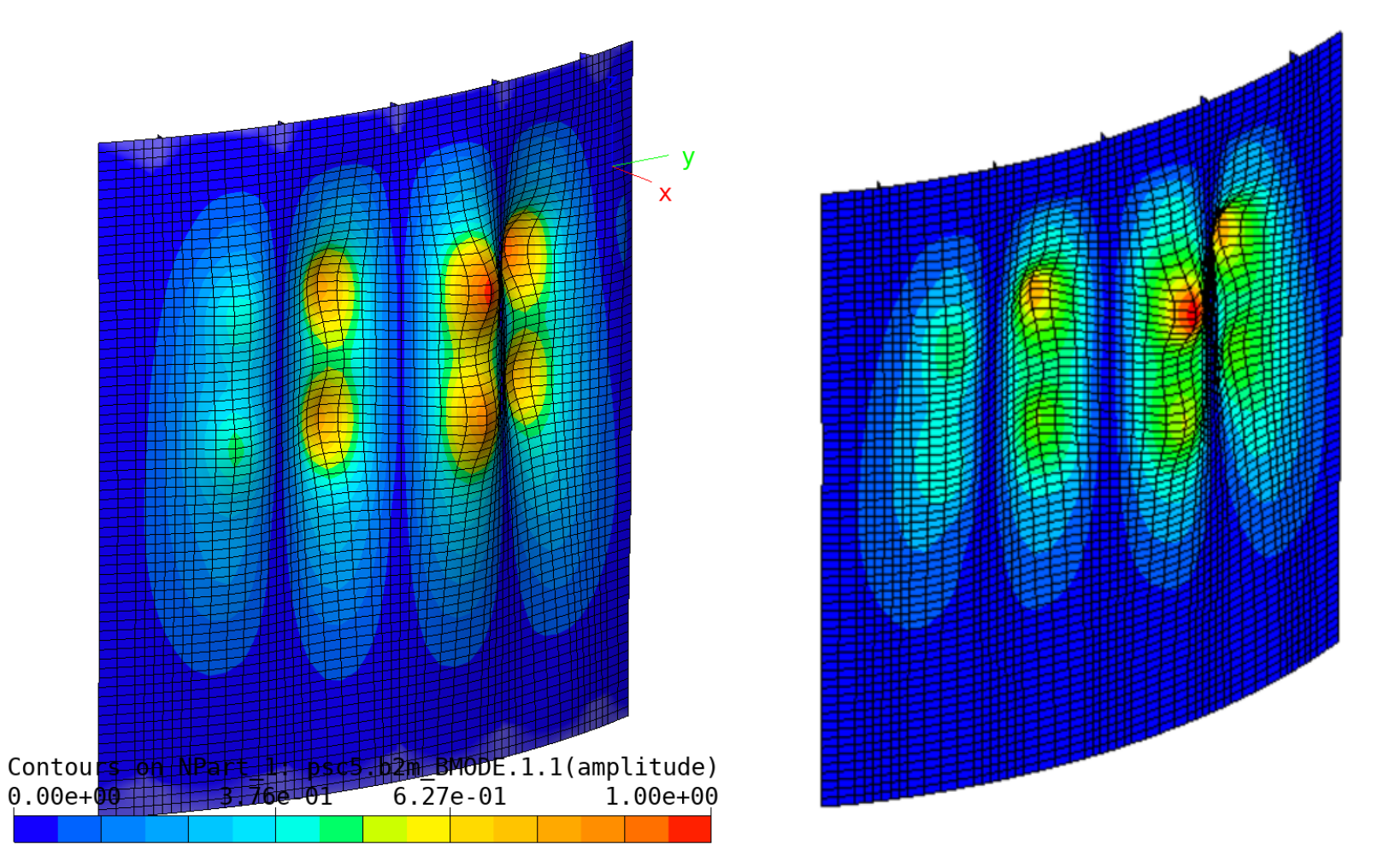
Left: B2000++ mode 1 (Pcrit=74.3 kN). Right: Abaqus mode 1 (Pcrit=75.8 kN).
The static solution up to a load factor of 3, i.e. an end shortening of 3mm, is obtained with solving for case 2:
b2000++ -define case=2 psc5.mdl

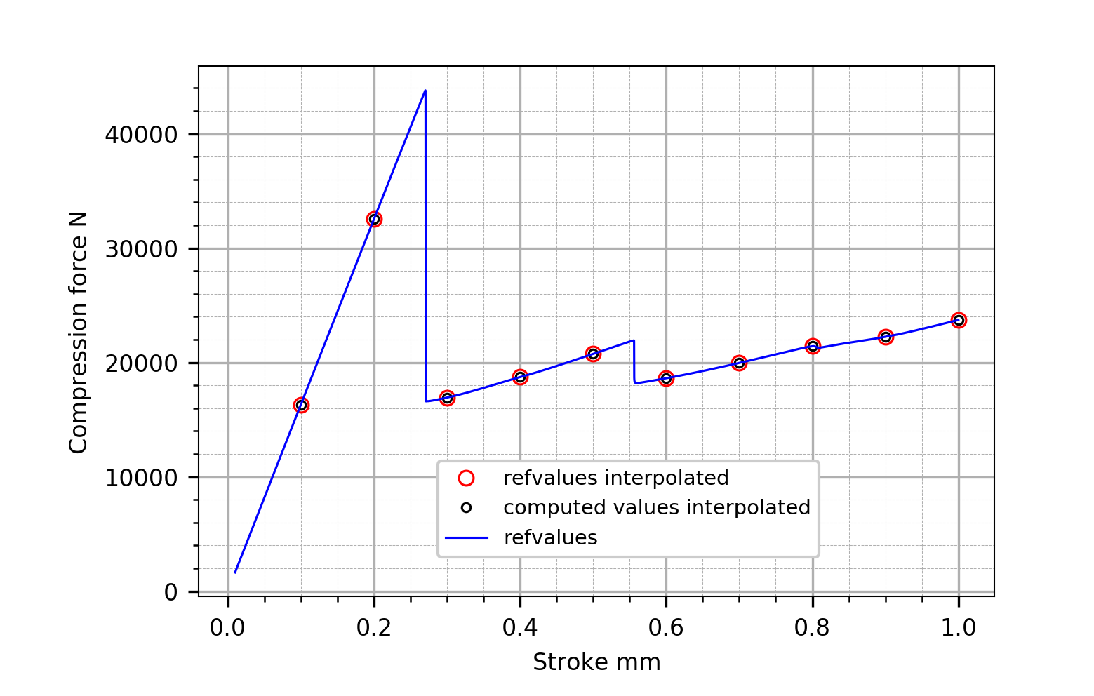
COCOMAT panel: Load step vs edge shortening curve (static analysis
case 2), generated with the rcurve.py script.
COCOMAT panel: Panel deformed shape of the last step. Note that the global buckling mode has developed at around 135 kN.
The implicit dynamic (transient) solution, obtained with the Nordsieck solver, gives the dynamic buckling solution - a more accurate solution, exhibiting intermediate buckling states:

COCOMAT panel: Comparison of static solution (black curve) and transient solution (red curve).
2.2.12. Cylindrical Panel (Verolme)
Note
Location of b case:
verification/solid_mechanics/buckling/verolme_panel
This test case is a variant of the panel described by Verolme [verolme1995] and Remmers [remmers1998]. The panel illustrates the post-buckling behaviour of an initially un-deformed panel, which ‘jumps’ from its pre-buckling state to a stable post-buckling state. Remmers [remmers1998] simulates the behavior by preforming a dynamic (transient) analysis at a load just after the instability point, following the mode-jumping technique according to Riks and Rankin [riks1996], [riks1997].
The term mode jumping is often used to describe a sudden dynamic change in a static process. In computational mechanics, the abrupt change in wave numbers (such as from pre- to post-buckling state) is indicated as a mode-jump. This phenomenon was first mentioned by Stein [stein1959], describing a buckling experiment with a flat panel. Mode-jumping is an important phenomenon for stiffened panels, where a mode-jump may occur from local skin buckling (between the stiffeners) to a global buckling pattern.
In order to simulate such jumps with FEA, one can use a transient solving routine including some form of damping, such as Rayleigh damping, in order to find a stable static path [2]. The artificial damping scheme of B2000++ allows for finding a stable path with ‘static’ analysis. This test case uses this artificial damping method to find a stable post-buckling solution (a non-damped simulation will fail).
The panel is made out of 2024-T3 aluminum and simply supported at the straight edges and clamped at the curved edges, as shown in the figure below. The panel is compressed at one of the curved edges, creating an edge shortening of 3 mm.

Geometry of Verolme panel
The geometry and material parameters are listed below:
Panel length \(L=0.5 m\), \(W=0.356 m\)
Panel radius \(R=0.38 m\), panel thickness \(t=0.001 m\)
Young’s modulus \(E=73.1 GPa\), Poisson ratio \(\nu=0.33\)
The numerical model for the test case uses a mesh of 20x20 elements. This will execute quickly, but is too coarse for an accurate result. An 80x80 mesh will produce an accurate result. Higher mesh densities do not show any significant improvement.
The following options are defined in the cases command:
cases
  case 1
    residue_function_type      artificial_damping
    dissipated_energy_fraction 2.e-6
    step_size_init             0.01
    step_size_max              0.005
    step_size_min              1e-13
    max_newton_iterations      30
    max_divergences            1
    increment_control_type     load
  end
end
The figure below shows the deformed panel and the load-shortening curve of the analysis for a 160x160 mesh and the load-shortening curves for other mesh densities.
Load-shortening curves for different mesh densities
2.3. Transient (Dynamic) Analysis
2.3.1. Forced Vibration (Bar)
Note
Location of verification case:
verification/solid_mechanics/dynamic/forced_vibration_bar
This case tests both the sfunction and the stabulated options
for prescribing time-dependent natural boundary conditions nbc,
i.e for the present case, time-dependent excitation forces.
A single DOF system is subject to a sinusoidal excitation force in the
global x-direction in the geometrically linear range. The theoretical
solution can be found in the text book by Clough and Penzien and is
displayed in the figure below. The code is contained in the test file
__init__.py.
The corresponding FE problem is formulated with 1 or several rod
elements in the x-direction in a line. All DOF’s except DOF 1 are
removed for all nodes. The mass is concentrated at the end node and
introduced with a PMASS3 element. The linear dynamic solver is
selected, since the problem is linear. Setting the
multistep_integration_order to 2 is the sufficient, the
numerical damping being dependent on the time step only. Check with
the input file r2_tabulated.mdl for the definition of the time
step.
The test checks forced vibration defined by the the case option
nbc, sfunction defining the excitation function with an
expression
nbc 1 sfunction 'sin(6.6666666666667*t)'
or stabulated with pairs (time, value):
nbc 1 stabulated [ 0.0 0.0 ... 2.4740042147 -0.707095118523 ]
Both options define the same sinusoidal excitation function of the natural boundary condition. The response is displayed below:
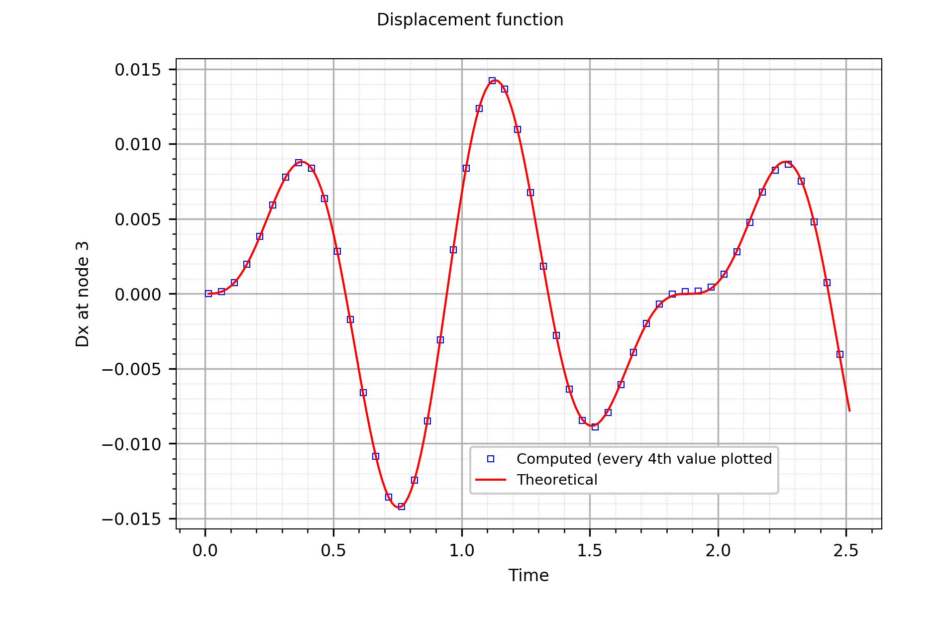
Time-displacement response function.
2.3.2. Nonlinear 1 DOF system
Note
Location of verification case:
verification/solid_mechanics/dynamic/one_dof_nonlinear
This simple rod snap problem consists of two rods. The FE model is show below. The rod dimensions are B=H=10 and the sections are circular with a radius of 0.5641896, i.e. a cross section area of 1.0. The material is linear isotropic with a modulus of elasticity E=1.e6. The rods are restrained at nodes 1 and 3, node 2 being free to move in the x- and y-direction, and the node 2 is initially deformed to 1 at time 0 and released. The example has been described by Argyris et.al [1], where the analytical formulation of the equation of motion of the two rod system can be found.
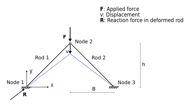
Non-linear one-dof problem: FE model and dimensions.
The figure below plots the FE solution (node 2, dof 2) vs the analytical one:
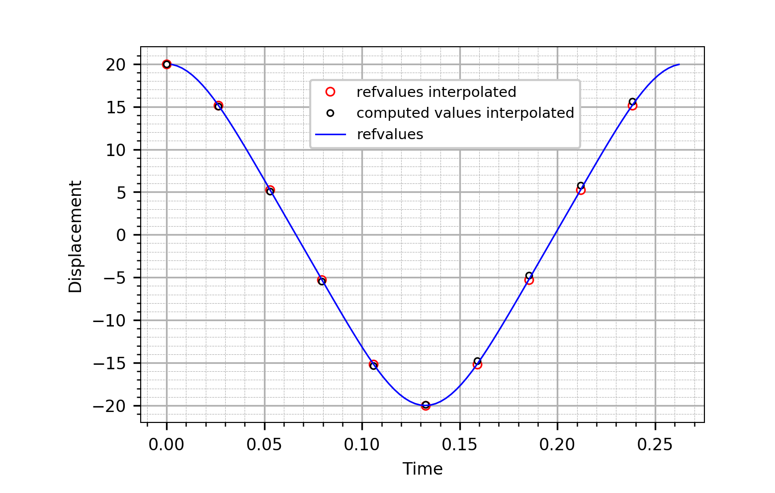
2.3.3. Cube in Gravitational Field
Note
Location of verification case:
verification/solid_mechanics/dynamic/one_element_gravity
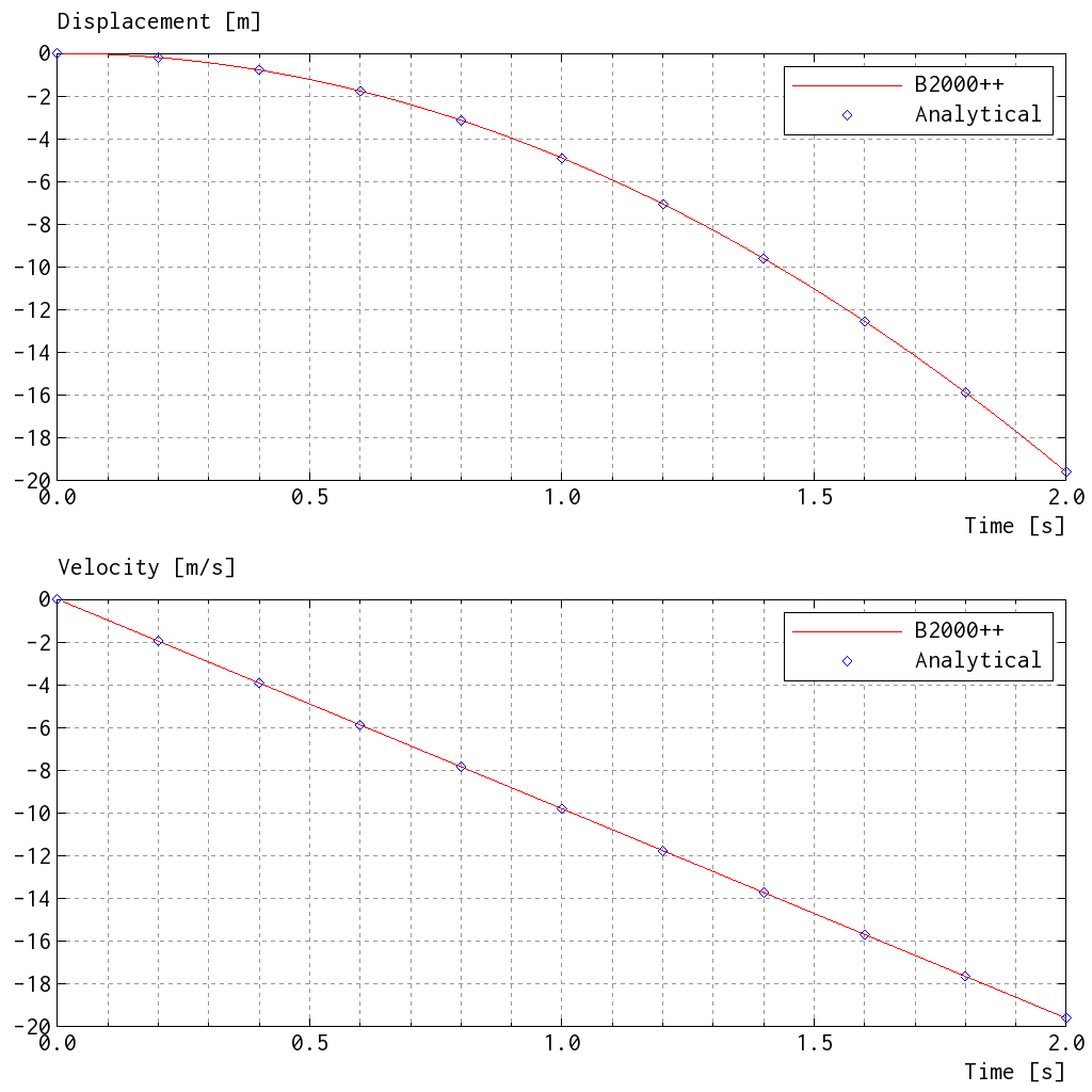
A solid cube is placed in a gravitational field g=(0, 0, -9.81) at time t=0 and released. The cube must move in ‘free fall’ along the negative z-axis with
and with the falling speed \(v = g_zt\), the acceleration \(a = g_z\) being constant. The model consists of HE8.S, HE20.S.TL, or HE27.S.TL elements. Different mesh densities are tested. The figure below displays the displacement, velocity, and acceleration functions for an integration time of 2s (solid lines are theoretical values).
The dynamic solution is relatively sensitive with respect to the error
tolerance. Relevant tolerances of the case option (see input file
he.mdl)
tol_residuum 2e-3
tol_solution 1e-4
have been found to lead all element types to convergence.
2.4. Free Vibration
2.4.1. Cylindrical Panel
Note
Location of verification case:
verification/solid_mechanics/freevibration/cylindrical_panel_1
The eigenfrequencies and eigenmodes of a thin isotropic cylindrical panel are calculated. The purpose of the analysis is to examine the performance of the MITC shell elements combined to point mass elements (PMASS).
The panel is supported with four springs attached to the corners of the plate. Thus, the panel is not fully constrained and a shift of 1.0 has to be applied in order to be able to solve the eigenvalue problem.

Cylindrical panel: Mesh (0 by 14 Q4 elements or 5 by 7 Q8/Q9 elements).
The panel has a length a = 1.039_m, radius R = 1. m, an angle φ = 49.4 and a thickness t = 0. m. The springs have a height h = and a cross section area of 1. m2. The materials are linear isotropic and the properties for the springs and the panel are listed below.
Panel: E=74e9 MPa, Poisson=0.3, density=2700 kg/m3
Springs: E=730 MPa, Poisson=0.3, density=0.024 kg/m3 0. 0.024
The free vibration analysis reveals that the first 6 eigenfrequencies are due to the vibration of the panel on its foundation. Therefore, only the 7th to 10th eigenfrequencies are listed in the table below:
Element |
Mode 7 |
Mode 8 |
Mode 9 |
Q4.S.MITC |
9.94 |
12.9 |
22.6 |
Q8.S.MITC |
9.93 |
12.7 |
22.4 |
Q9.S.MITC |
9.91 |
12.7 |
22.4 |
Cylindrical panel: Mode 7 (left) and 8 (right).
2.4.2. Eigenfrequencies of Hinged Plate
Note
Location of verification case:
verification/solid_mechanics/freevibration/hinged_plate
The eigenfrequencies and eigenmodes of a thin flat isotropic plate
with a hinge are calculated. The purpose of the analysis is to
demonstrate and check the modelling of a hinge, by means of different
patches and the LINC command. Mass matrices are calculated with
the default B2000++ consistent mass configuration.
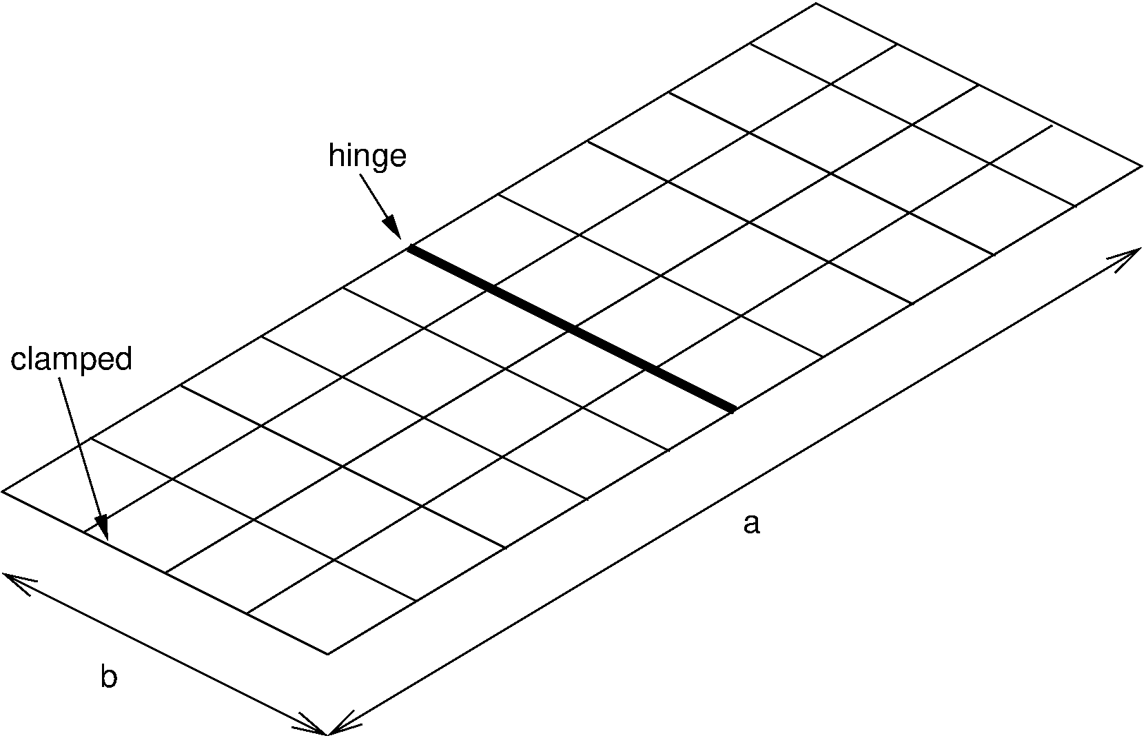
Flat isotropic plate with hinge
The plate has a total length of a = 1.0 [m], a width b = 0.4 [m] and a thickness t = 0.004 [m]. The material of the plate is linear isotropic with a modulus of elasticity E = 74.E9 [N/m:sup:2], a Poisson number ν = 0.3 and a density ρ = 2700 [kg/m:sup:3]. One of the short edges is clamped, while the others are free. The hinge is located halfway between the two smaller edges (at a = a/2). The input options are listed below.
|
Selects the hinge type: htype=1 adds a hinge, htype=2 means no hinge. |
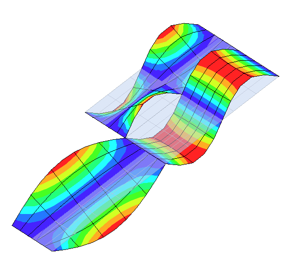
The results for the different element types for the plate with or without hinge are listed in the table below:
Element |
Hinge |
f1 |
f2 |
f3 |
f4 |
f5 |
Q4.S.MI TC.E4 |
yes |
3.46 |
17.84 |
21.56 |
56.76 |
60.77 |
Q4.S.MI TC.E4 |
no |
9.73 |
17.79 |
54.88 |
60.75 |
84.20 |
2.4.3. Eigenfrequencies of Flat Isotropic Plate
Location of verification case: $B2VERIFICATION/solid_mechanics/freevibration/isotropic_plate
The eigenfrequencies and eigenmodes of a thin flat rectangular isotropic plate are calculated for MITC shell elements with 4, 8, and 9 nodes. The plate has a length a = 10 m, width b = 0.4 m and a thickness t = 0.002 m. The material is linear isotropic, with modulus of elasticity E = 72 MPa, Poisson number 0.3, and density 2400 [kg/m3]. The edges I and III are simply supported. The other two edges are free. The plate is modeled using a regular 10 by 10 element mesh.

Flat isotropic plate (10 by 10 element mesh)</title>
Analytical solutions can be obtained from various sources, and
computed values are not listed here (see __init__.py). The
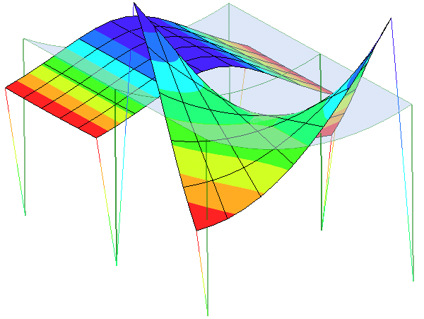
figure below shows the second, third, and fourth eigenmode of the
plate with respect to the initial shape.
f1 |
f2 |
f3 |
f4 |
5.0 |
17.1 |
20.2 |
38.6 |
Mode shapes for different eigenvalues</title>
2.4.4. Composite Panel with Stringers
Note
Location of verification case:
verification/solid_mechanics/free_vibration/panel3
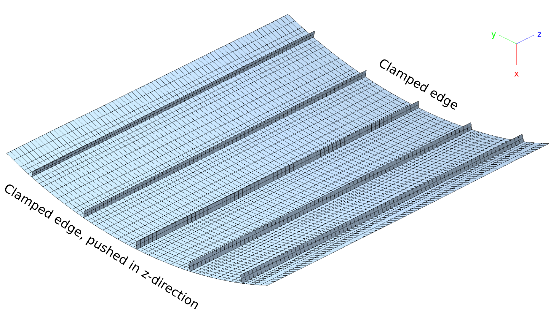
The three string composite panel is a test case for demonstrating the B2000++ capabilities of dealing with lightweight composite structures modeled with shell or solid elements. A cylindrical panel with 3 stiffeners is subjected to axial compression load. The free vibration modes are to be determined under zero compression load.
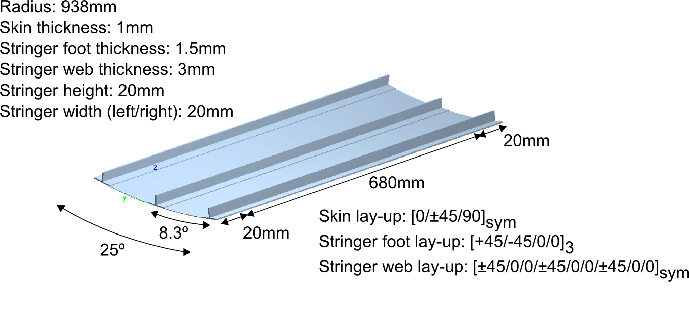
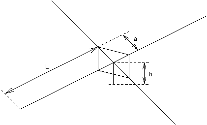
Three Stringer Composite Panel: Dimensions and laminate setup.
The boundary conditions are displayed in the figure below: Both curved
edges are clamped and both straight edges are free. One of the curved
edges is pushed towards the panel, causing it to buckle. All boundary
conditions are essential boundary conditions (ebc command in the
MDL input files).
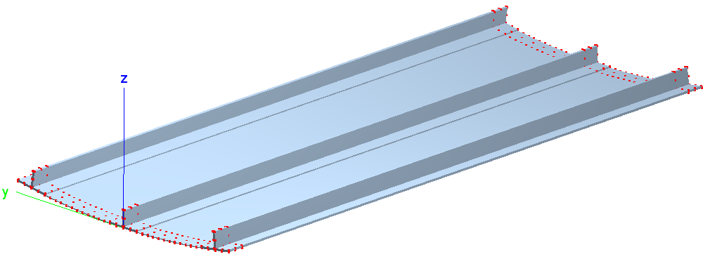
Three Stringer Composite Panel: Boundary conditions at nodes (red dots).
The shell model consists of Q9 MITC shell elements. The cylindrical shell and the shell plus the stringer foot are modeled with one element through the thickness, as is the stringer. The laminate orientations and laminate placement are visualized with baspl++:
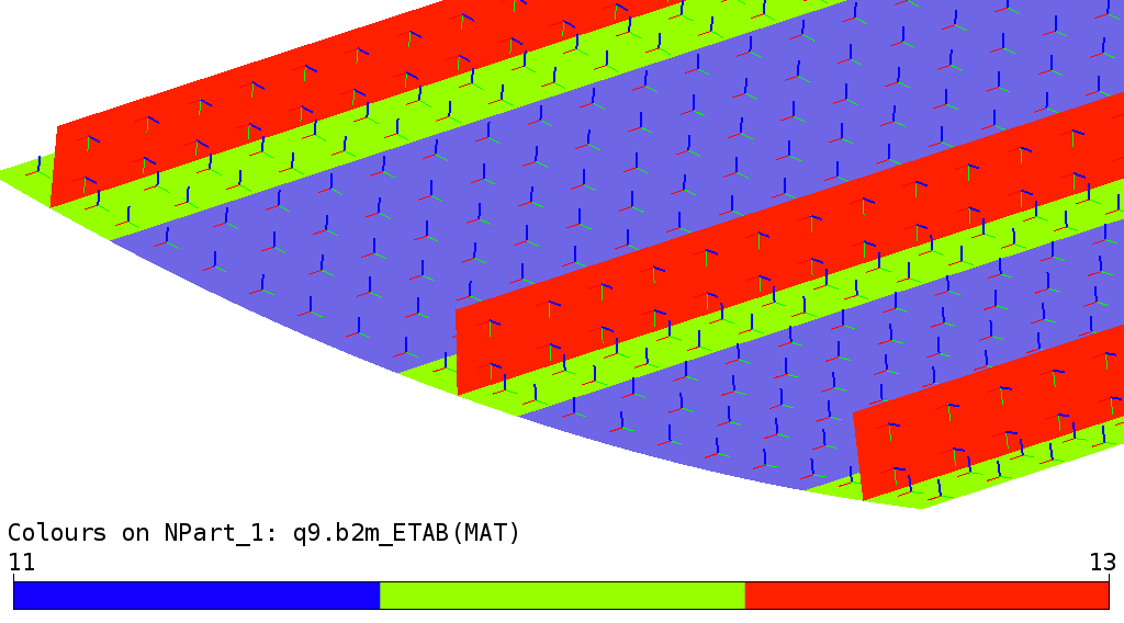
Three Stringer Composite Panel (solid model) : Laminates and material axis x (red) and y (green). Laminate 1 is material 11 (blue), laminate 2 is material 12 (yellow), and laminate 3 is material 13 (white).
Free vibration modes and their eigenfrequencies of the panel without prestress of the shell model are computed for load case 1, requiring the first 10 modes:
case 1
  ebc       1
  analysis  free_vibration
  nmodes    10
  gradients 1
end
The analysis of the shell composite model is launched by the shell command
prompt> b2000++ --adir 'cases=1' -l "info of solver in cerr" shell.mdl
Eigenfrequencies can be extracted and printed with
b2print_eigenfrequencies and plotted with the baspl++
script view_vibration_modes.py.
b2print_eigenfrequencies shell

Eigenfrequencies, case 1
     Mode         FREQ        OMEGA         MODK         MODM
        1        205.3         1290        116.1    6.979e-05
        2        268.7         1688        339.5    0.0001191
        3        304.3         1912        497.9    0.0001362
        4        308.4         1938        364.3    9.703e-05
        5        349.6         2197        425.2    8.813e-05
        6        380.1         2388        296.5    5.198e-05
        7        434.7         2731        774.1    0.0001038
        8        508.5         3195        448.3    4.392e-05
        9        547.4         3439        414.3    3.503e-05
       10        606.4         3810         1027    7.073e-05
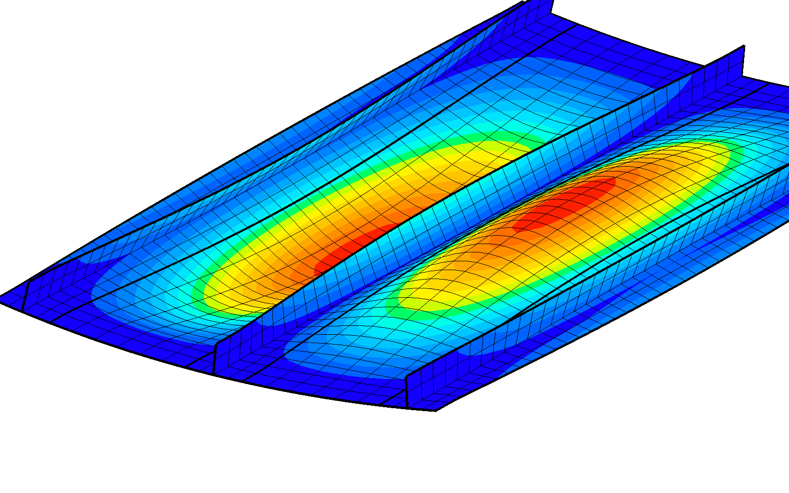
Three Stringer Composite Panel (shell model): First vibration mode mode.
Similarly, the analysis of the solid composite model is launched by the shell command
prompt> b2000++ --adir 'cases=1' -l "info of solver in cerr" solid.mdl
Eigenfrequencies can be extracted and printed with
b2print_eigenfrequencies and can be plotted with the
baspl++ script view_vibration_modes.py.
b2print_eigenfrequencies solid

Eigenfrequencies, case 1
 Mode    Frequency        Omega      Modal_K      Modal_M
    1        205.5         1291    7.086e-05        118.1
    2        265.5         1668    0.0001237        344.4
    3        303.5         1907    0.0001339        486.9
    4        305.6         1920    8.978e-05        331.1
    5        351.4         2208    8.546e-05        416.6
    6          383         2407    5.331e-05        308.8
    7        439.7         2763     0.000104        793.9
    8        513.2         3225    4.565e-05        474.7
    9        554.8         3486    3.647e-05        443.1
   10        613.7         3856    7.478e-05         1112
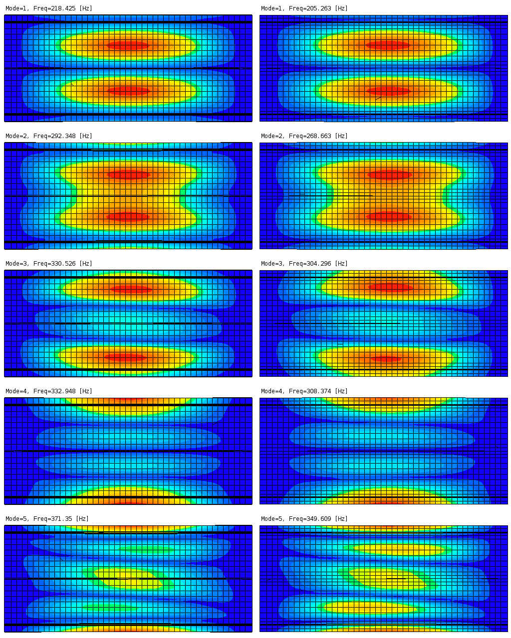
Three Stringer Composite Panel (shell model): Comparison of eigemodes. Shell model (left column) and solid model (right column).
2.4.5. PMASS free vibration tests
Note
Location of verification case:
verification/solid_mechanics/freevibration/pmass1
This free vibration tests check the PMASS3 point mass elements. The test compute the first n eigenfrequencies of a clamped beam with a consistent mass matrix or with equivalent PMASS3 elements:
beam.mdl: Consistent beam element mass formulation.pmass3.mdl: PMASS3 point masses lumped at the mesh nodes. The density of the beam elements is then set to 0. Note that the PMASS tests are performed with B2 elements only, the B3 elements not being suited for this type of test because of the extra node.
The beam dimensions can be consulted in the params.mdl file. The
material is isotropic, and the beam is modeled with B2.S.RS elements.
The test compares all configurations, which must give the same result.
2.4.6. PMASS6 free vibration tests
Note
Location of verification case:
verification/solid_mechanics/freevibration/pmass2
This free vibration tests check the PMASS6 point mass elements. The tests compute the first n eigenfrequencies of a clamped beam with various configurations of PMASS6, or equivalent RBE elements. The beam is massless and acts as a spring for the PMASS6 and RBE elements.
Clamped beam with PMASS3, PMASS6, or RBE element at the tip.
Clamped beam with a PMASS6 or RBE element at the tip with an offset y in the x-y plane (DOF’s 3 4 5 eliminated) and with an offset in the x-z plane (DOF’s 2 4 6 eliminated).
Clamped beam with a PMASS3 element at the tip with an offset in y simulated by a rigid beam.
The beam dimensions can be consulted in the params.mdl file. The
material is isotropic, and the beam is modeled with B2.S.RS elements.
The mass is a cube of dimensions LX*LY*LZ and density RHO2 (see
params.mdl) and is modeled with a single HE8 elemen (for the RBE
tests).
The test compares equivalent configurations, i.e. PMASS6 vs. RBE without offset and PMASS6 vs. RBE with and offset.
2.4.7. Prestressed Beams
Note
Location of verification case:
verification/solid_mechanics/freevibration/prestressed_beams
The eigenfrequencies and eigenmodes of a simplified helicopter rotor modeled with beam elements are calculated. The rotor consists of four blades connected to each other by springs.
Helicopter rotor model
The geometry data as well as the material properties (all isotropic elastic) are listed below:
\(length L=1.7m\) \(area A=0.01m^2\) \(head width a=0.2m\) \(shaft height h=0.1m\) \(Iyy=Izz=2.8e-8m^4\) \(Ip=2*Iyy\) \(Sy=Sz=100m^2\)
\(E_rotor=1.E10{N/m^2}\) \(\rho_rotor=117.6{kg/m^3}\) \(E_springs=1.E6{N/m^2}\) \(\rho_springs=100{kg/m^3}\)
The end point of the shaft is fully clamped.
he solutions are independent of the mesh type or join type and vary only due to the prestress. The table below lists the 10 lowest eigenfrequencies.
Prestress |
1st |
2nd |
3rd |
4th |
5th |
0.0 |
2.987 |
2.987 |
2.987 |
2.987 |
2.987 |
1E7 |
44.178 |
44.189 |
44.189 |
44.189 |
44.189 |
Prestress |
6th |
7th |
8th |
9th |
10th |
0.0 |
3.1136 |
3.1138 |
3.197 |
18.643 |
18.643 |
1E7 |
44.3967 |
44.3972 |
44.590 |
130.31 |
130.35 |
1st and 4th eigenmode as well as the initial shape. Notice that the first 5 eigenfrequencies are virtually the same, as are the 6th, 7th and 8th eigenfrequencies and the 9th and 10th.
The input options to the test program are:
meshtype: Type of mesh to be generated: meshtype=1 selects one branch, meshtype=2 selects four branches.
jointype: Branch join type: jointype=1 selects automatic join, jointype=2 selects manual join (meshtype=2 only).
prestr: Specifies the value of the prestress: Analysis is performed with prestr=1.0e7) or without prestress (prestr=0).
2.5. Material Failure
2.5.1. Hashin Criterion Failure Envelope
Note
Location of verification case:
verification/solid_mechanics/failure/hashin
The Hashin criterion [hashin80] failure envelope for \(\sigma_{22}\) vs \(\sigma_{12}\) is computed with one single HE solid element by executing B2000++ runs with displacement constraints corresponding to the desired stress state. The results are compared to data from literature [pinho].

Note: The Hashin failure criterion data are entered with the
failure subcommand of the MDL material command. Example from
test:
failure hashin
   t1  1000. # (not used)
   c1  1000. # (not used)
   t2  37.5
   c2  130.5
   s12 66.5
   s23 49.09 # equation 68 in [pinho] = 0.378 * c2
end
2.5.2. Solid Elements Rod
Note
Location of example case:
verification/solid_mechanics/kinematic_coupling/pulled_rod_solid_elements
A rod meshed with HE8 solid elements and composed of two sections with two different square cross section areas is clamped at one end and pulled at the other end. The two sections are coupled with the common mesh refinement kinematic coupling method of B2000++. The analysis is linear. Square areas with an area ration of 5:1 and 2.5:1 are checked, the first section area always being the same and the second one being varied.

Mesh and boundary conditions
The analytic reference solution for the displacement \(u_x\) at \(x=2L\) is simple, since the model is ‘statically determined’:
Displacements in the x-direction agree within 0.01% with the analytic solution.
2.6. Model Reduction
2.6.1. Vibration of a Clamped Beam
Note
Location of verification case:
verification/solid_mechanics/model_reduction/beam
The test computes vibration modes of a clamped beam with the Component Mode Synthesis method (also referred to as the Craig-Bampton method) global-local analysis method. The analysis consists of 2 steps, one with a global coarse mesh, and one with a local fine mesh. In a first step the global model is reduced to a macro-element. Then, the local model uses this reduced system defined by the global model for making a local (detailed) vibration analysis.
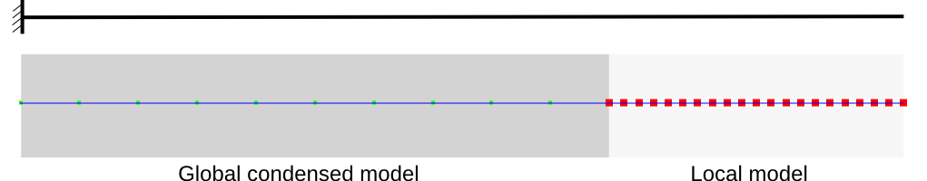
Clamped beam global-local model.
The global-local analysis is performed as follows:
Condensate the global model
x_global.mdl.Create the input database of the local model
detail.mdl.Update the input database of the local model with the information from the global model. This step has to be performed with a Python script (here:
b2ipupdate.py).Compute vibration modes with the local model.
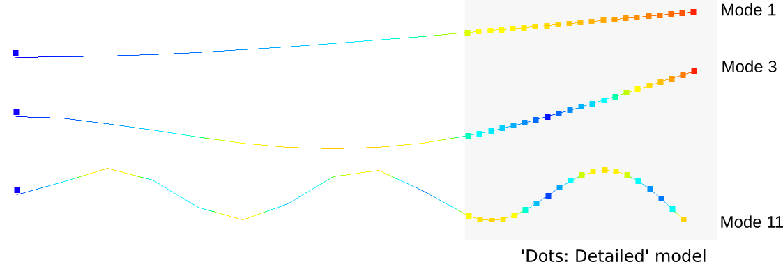
Vibration mode shapes. Dots: Local model. Solid line: Global reference model.