3. Heat Flow Analysis

3.1. Stationary Heat Flow

3.1.1. Heat Conduction

3.1.1.1. One-Dimensional Test

Folder: B2VERIFICATION/heat_flow/basic/conduction/basic

These tests check the 2D and 3D heat flow conduction elements with linear heat conductivity in one dimension. Given a wall that extends infinitely in the y- and z-directions, the tests compute the temperature through the wall in x-direction.

Case 1 specifies temperatures at the wall surfaces \(T(x=0)=T_1\) and \(T(x=L)=T_2\). For a temperature-invariant thermal conductivity the theoretical solution is

\[T(x) = T_1 + (T_2 - T_1) \frac {x}{L}\]

where \(T_1\) is the wall temperature at x=0, \(T_2\) the wall temperature at x=L, and L the wall thickness. The constant heat flux is

\[q = -k (T_2 - T_1) \frac {(T_2 - T_1)}{L}\]

T, Q, HE, TE, and PR regular and skew elements are tested, the problem being the same in case of 2D or 3D elements. The figure below shows the model and the temperature distribution for the H20 case (4 elements)

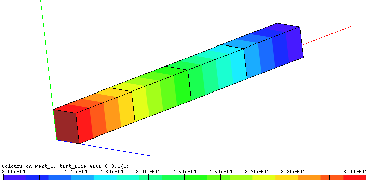
Case 1: Temperature distribution through Wall. Wall surface temperatures fixed.

Case 2 specifies temperatures at the wall surfaces \(T(x=0)=T_1=20\) and \(T(x=L)=T_2=20\) and the wall is heated internally with a constant heat source w. For a temperature-invariant thermal conductivity the theoretical solution is

\[T(x) = T_1 - \frac{0.5 w x^2}{k} + \frac{(T_2 - T_1)x}{L} + \frac{0.5 w L x}{k}\]

where k is the thermal conductivity. The figure below shows the model and the temperature distribution for the H20 case (4 elements)

Case 2: Temperature distribution through Wall. Wall surface temperatures fixed and wall heated internally.

T, Q, HE, TE, and PR elements are tested, the problem being the same in case of 2D or 3D elements.

3.1.1.2. Heat Conduction in Tube

Folder: $B2VERIFICATION/heat_flow/stationary/conduction/tube_segment

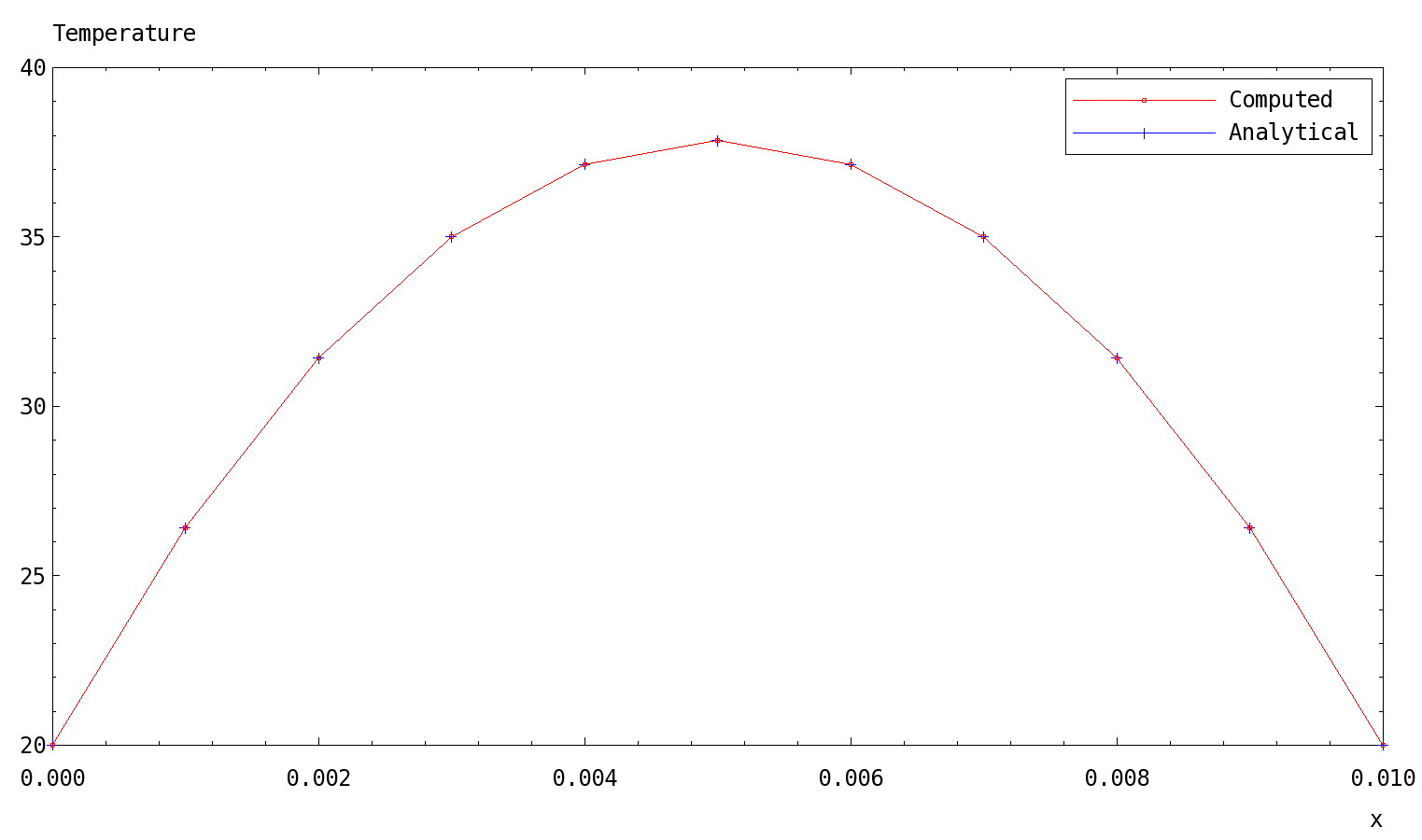
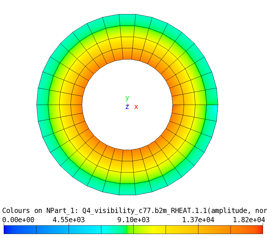
Compute the temperature distribution in a thick tube segment with linear heat conduction properties. The temperature is set to \(100^{\circ} C\) on the outer wall of the tube and \(0^{\circ} C\) on the inner wall of the tube. All other walls are isolated.

Tube mesh: Patch edges in red, inner wall solid gray.

Tube: Temperature distribution. Graph displays temperature through the wall.

3.1.1.3. One-Dimensional Test

Folder : $B2VERIFICATION/heat_flow/stationary/convection

These tests check 2D and 3D heat equation elements with linear conduction and convection in one dimension. In addition, expressions for the convection law are tested, too.

Given a concrete wall that extends infinitely in the y- and z-directions, compute the temperature through the wall. The wall at x=0 is exposed to air at 270K and the wall at x=L= to air at 330K. Both conditions are formulated with convection overlay elements. The convection coefficient for x=0 is \(h_{c1}=40W/m^2\), modeling an air current, and for x=L it is \(h_{c2}=10[W/m2/K\) modeling still air. The conduction coefficient k of concrete is set to \(1.8W/m/K\)

The theoretical solution for the heat flux through the wall is (see also Kreith & Bohn, Principles of Heat Transfer [kreith])

\[q = \frac{T_2 - T_1}{ \frac{1}{h_{c1}} + \frac{L}{k} + \frac{1}{h_{c2}}}\]

With the constants from above the heat flow through the wall becomes

\[q = \frac{270-330}{1/40 + 0.2/1.8 + 1/10} = -254.1\]

i.e. the heat flows from the right to the left in the figure below. Both Q and HE elements are tested, the problem being the same in case of 2D or 3D elements. The mesh for the 2D element model with Q4 conduction elements and L2 convection elements is displayed below:

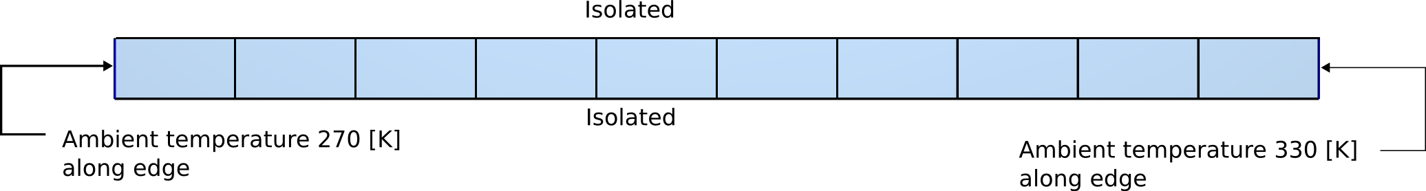
For the 2D cases the convection conditions are modeled led with L2 or L3 convection overlay line elements along the vertical edges of the above model. Please note that, for a 2D model the thickness, i.e. the extension of the model in the z-direction, must be specified both for the conduction and the convection overlay elements.

For the 3D cases the conduction in the solid is modeled with HE8 or TE4 elements and the convection conditions with Q4 or T3 convection overlay surface elements along the vertical faces of the model. Please note that the thickness of conduction and convection overlay elements is ignored!

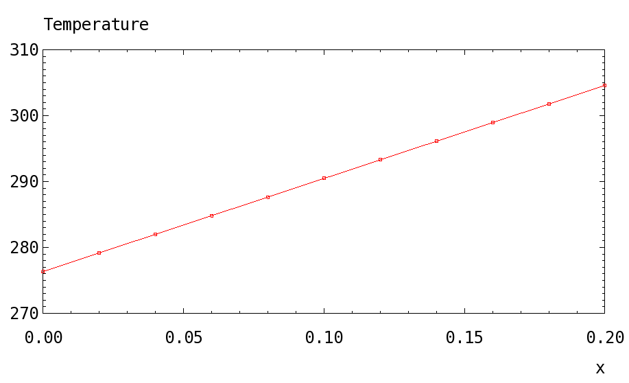
All tests give the same result for the heat flow, i.e. the element gradient in the x-direction, with a value of -254.1. The temperature distribution is, as expected, linear:

3.1.2. Radiation

3.1.2.1. Radiation of Cylinder to Plate

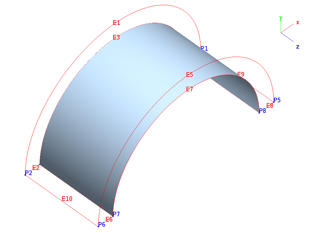
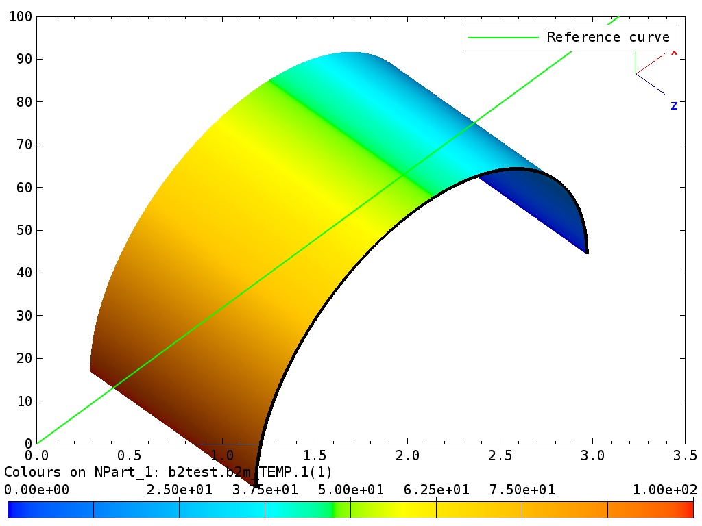
Folder: $B2VERIFICATION/heat_flow/stationary/radiation/cyl_plate

A cylinder steadily radiates heat on a plate. This example demonstrates the view factor capabilities of B2000++. An analytical solution is available for the view factor in the text book by Siegel and Howell [siegel].

The cylinder and the annular plate are meshed independently one of the other as shown in the figure below. If only radiation elements (Q4 elements) are used, the solution will consist of exchanged heat between the cylinder (hot) and the plate (cold). Since all nodes have prescribed temperatures there are no unknowns. However, B2000++ has to solve for the non-linear essential boundary conditions imposed by the radiation. Special attention has to be brought to the directions of the normals of the surfaces (see figure). If the normals are not oriented properly the structures will not radiate in the desired directions.

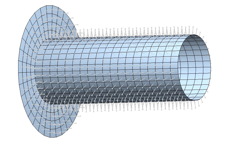
Radiation of cylinder to plate: Mesh and normals.

Radiation problems are nonlinear as specified in the adir command below. The linear transient response is calculated with the default non-linear solver of B2000++, with the parameters defined in the case command (see input file radiation_cyl_plate.mdl):

cases
   case 1
      ebc                      1
      component radiation_heat NBC VISI_RAD
      step_size_init           1
      step_size_min            1
      step_size_max            1
   end
end

adir
   analysis nonlinear
   case 1
end

By setting the initial step size, the minimum step size, and the maximum step size to 1, the solver will try to solve the problem for the final step with one step.

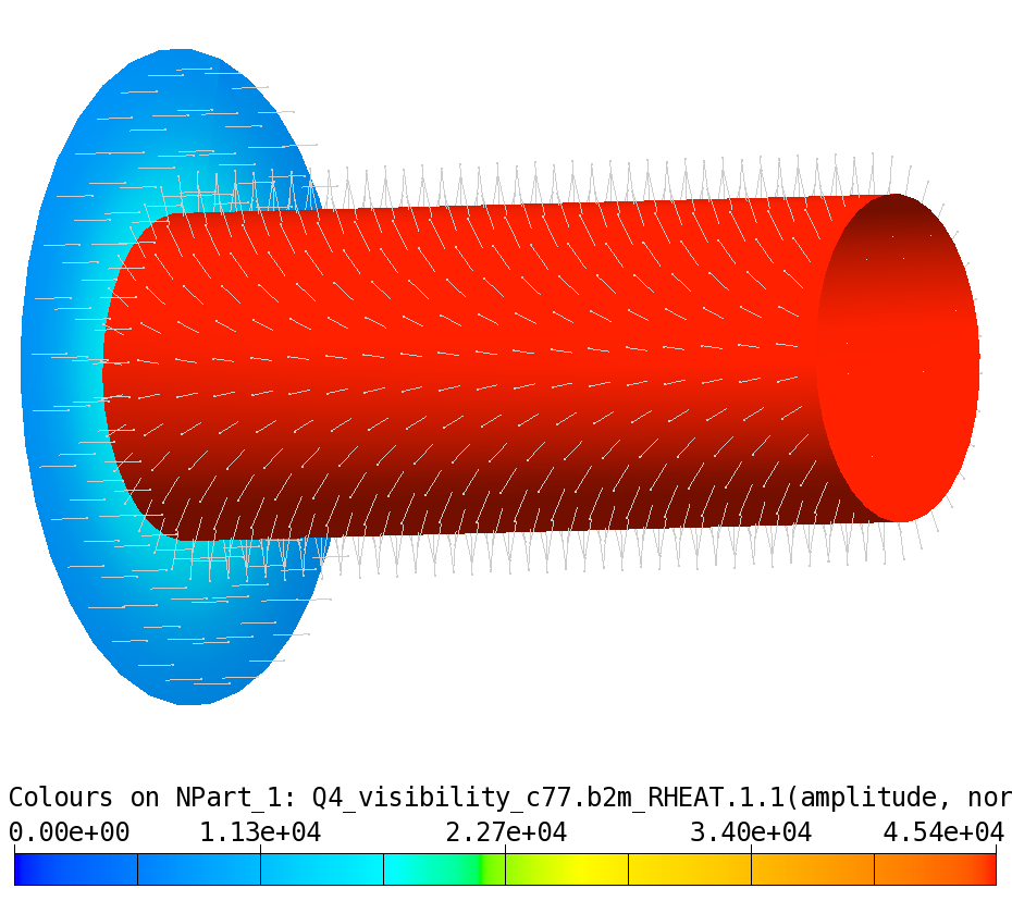
Radiation of a cylinder: Accumulated heat.

Radiation of a cylinder: Accumulated heat, detail (different scale).

The approximate analytical value for the radiation configuration factor based on pure geometric considerations can be found in the graph of the text book by Siegel and Howell. For the geometric configuration of present example the view factor is ~0.4.

3.1.2.2. Radiation of Heated Wire

Folder: $B2VERIFICATION/heat_flow/stationary/radiation/heated_wire

The test checks the 1D radiation overlay elements and demonstrates radiation capability of B2000++. A heated wire with surface temperature \(T_s\) is placed in a black body enclosure of temperature \(T_{inf}\). The heat flux \(q_s\) from the surface of the wire is then

\[q_s = s e (T_{s}^4 - T_{inf}^4)\]

where s is the Boltzmann constant (\(5.67 10^{-8} W/m^2/K^{-4}\)) and e the emissivity (here: 1.0), The wire material is copper (\(k=400 W/m\)) and the wire radius is 0.001 m.

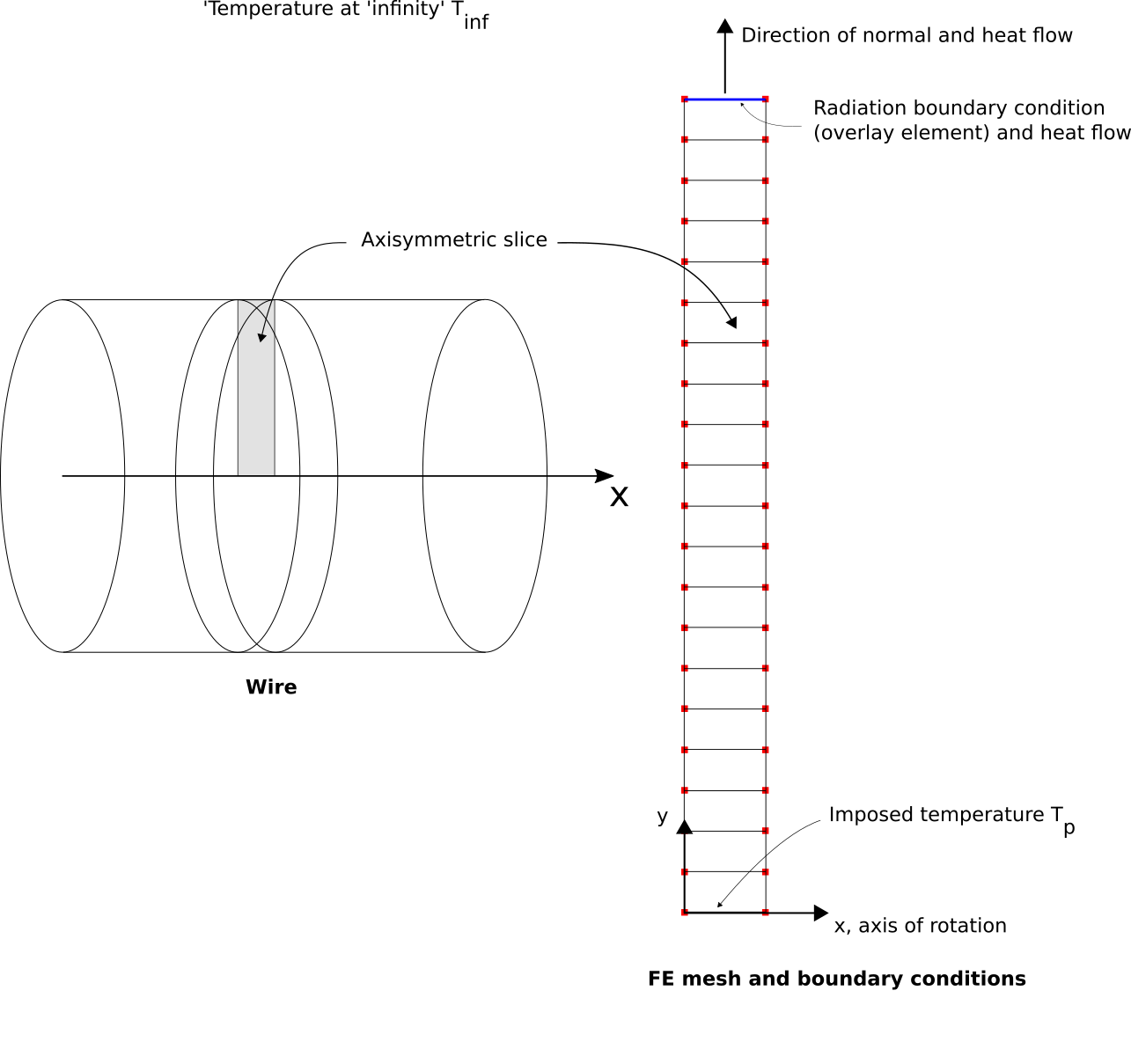
A slice one element wide is modeled with axisymmetric heat conduction elements. Boundary conditions are:

• Symmetry along the left and right side, which means ‘free’ edges, i.e. no ebc and nbc conditions applied.

• \(T=T_s\) in the body. Setting along y=0 will propagate \(T_s\) through the body.

• Radiation on the surface by applying radiation elements, see epatch 2 definition in the input file.

The test checks the heat flow \(q_s\) through the wire surface of the wire against the above solution by extracting the heat flow field HEAT_RADCONV for the top element and comparing the values to the theoretical ones.