7. Kinematic Coupling
7.1. Vibration of Clamped Beam (Craig-Bampton Method)
* TEXT TO BE REVISED STEPS WRONG *
Folder: $B2EXAMPLES/globallocal/beam
The test computes vibration modes of a clamped beam with the Component Mode Synthesis method (also referred to as the Craig-Bampton method) global-local analysis method. The analysis consists of 2 steps, one with a global coarse mesh, and one with a local fine mesh. In a first step the global model is reduced to a macro-element. Then, the local model uses this reduced system defined by the global model for making a local (detailed) vibration analysis.

The global-local analysis is performed with the run.py script
as follows:
Condensate the global model
global.mdl.Create the input database of the local model
local.mdl.Update the input database of the local model with the information from the global model. This step has to be performed with a Python script.
Compute vibration modes with the local model.
Eigenfrequencies can now be extracted from the global model:
$ b2print_eigenfrequencies --case=2 global

Eigenfrequencies, case 2
     Mode         FREQ        OMEGA         MODK         MODM
        1        3.726        23.41        480.8       0.8774
        2        11.17        70.21         4326       0.8777
        3         23.4          147         1857       0.0859
        4        65.76        413.2         5381      0.03152
        5        70.07        440.3    1.672e+04      0.08626
        6        129.6        814.2    1.051e+04      0.01586
        7        196.5         1235    4.822e+04      0.03162
        8        216.2         1359    1.728e+04     0.009362
        9        305.9         1922        506.5    0.0001372
       10        326.1         2049    2.491e+04     0.005934
For comparison, eigenfrequencies of the reference model:
$ b2print_eigenfrequencies --case=2 reference

Eigenfrequencies, case 2
     Mode         FREQ        OMEGA         MODK         MODM
        1        3.725        23.41        480.8       0.8775
        2        11.17         70.2         4326       0.8778
        3        23.35        146.7         1858      0.08637
        4        65.38        410.8         5404      0.03203
        5         69.9        439.2    1.673e+04      0.08675
        6        128.1        805.1    1.057e+04       0.0163
        7        195.2         1227    4.873e+04      0.03239
        8        211.9         1331    1.746e+04     0.009849
        9        301.5         1895        524.9    0.0001462
       10        316.7         1990    2.606e+04     0.006582
Modes 2,5 and 7 are displayed in the montage plot below (the modes are
extracted and displayed with the baspl++ script view.py and
merged with the montage utility.
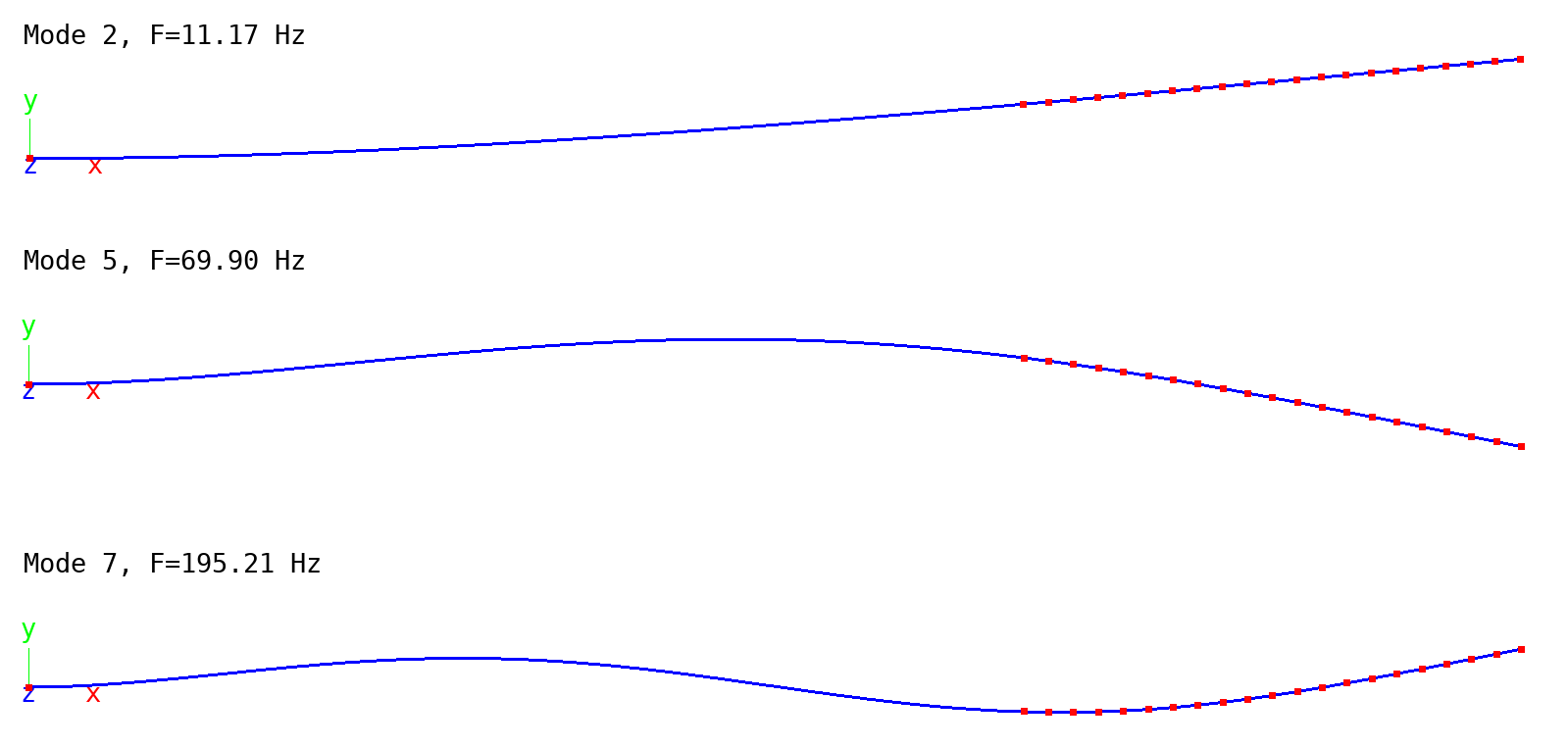
Some vibration mode shapes. Dots: Local model. Solid line: Global reference model.
7.2. I-Profile Beam
Folder: $B2EXAMPLES/globallocal/tying
This examples illustrates coupling of non-matching meshes. An I-profile beam subjected to thermal loading is modeled with solid elements. The 2 flanges and the web are modeled separately and ’tied’ together to form the complete model, referred to as ’tie’ model. The figure below the shapes of the separate models (B2000++ epatches). It also show the interfaces to be ’tied’, i.e. the lower and upper faces (black dots) of the web (green shape), which are ’tied’ to the corresponding faces of the lower and upper flanges.
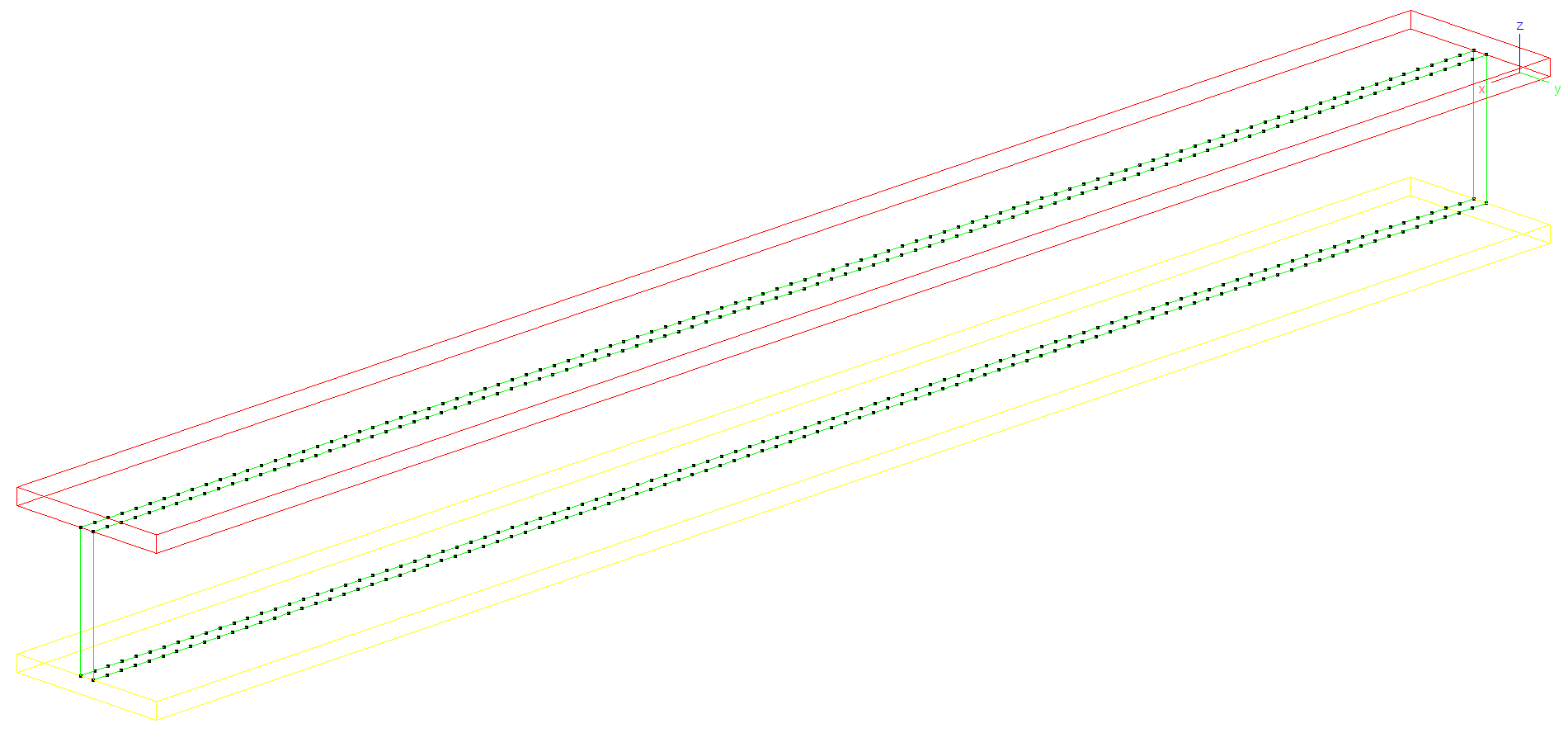
Mesh: Element pach contours of lower flange (yellow), web (green), and upper flange(red). Tie interface points shown in black.
To get reference solutions, the same model is assembled to a single
continuous mesh with the B2000++ join option. The continuous mesh,
however, can be generated only if the nodes of the interface are
matching. This is the case for mesh A (see below).
Results are compared to a model with a single matching mesh (join
model) and to analytical results from beam theory.
7.2.1. Meshes
Mesh A is selected such that the mesh nodes at the interface are matching, thus allowing for direct comparison of the tie and join models. The figure below displays the continuous mesh A of the structure.
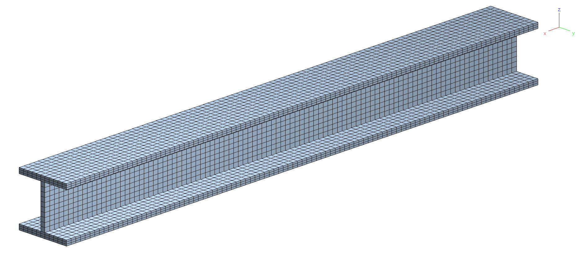
HE (hexahedral) mesh of continuous model (meshA).
Mesh B is selected such that the mesh nodes at the interfaces are not matching and thus can be used with kinematic coupling only. The quality of the solution is then compared to mesh A. The mesh density of the web of mesh B in x-direction is 66% of the one of mesh A.
7.2.2. Coupled Static Heat-Deformation Analysis
The couple static heat and deformation analysis is performed in 2 steps, a heat analysis followed by a deformation analysis retrieving the temperature distribution of the previous heat analysis.
The heat analysis boundary condition sets the upper flange of the structure to 100 °C and the lower on to 0 °C.
Several deformation analysis boundary conditions are studied:
Condition C1 clamps the beam at x=0. This creates bending with the give temperature distribution. It is interesting to note that (1) the deformations for this case, at least with beam theory, are independent of the cross section shape, the only intervening parameter being the height and that (2) the beam is stress-free, since it can deform freely. This case has a simple beam theory solution for the beam tip displacement.
Condition C2 clamps the beam at x=0 and X=L, thus generating stresses.
Results for condition C1 are summarized in the table below, demonstrating the efficiency of the kinematic coupling method, the tip displacements obtained with the 3 methods being practically identical.
Method |
z-displacement |
|---|---|
Mesh A: Join (matching) |
|
Mesh A: Tie (kinematic coupling, matching meshes) |
|
Mesh B: Tie (kinematic coupling, non matching meshes) |
|
Beam theory |
|
Global solutions for the heat analysis and the subsequent deformation analysis for condition C1 and mesh B non-matching) are displayed in the figures below. Stresses in the whole model are 0, as expected.
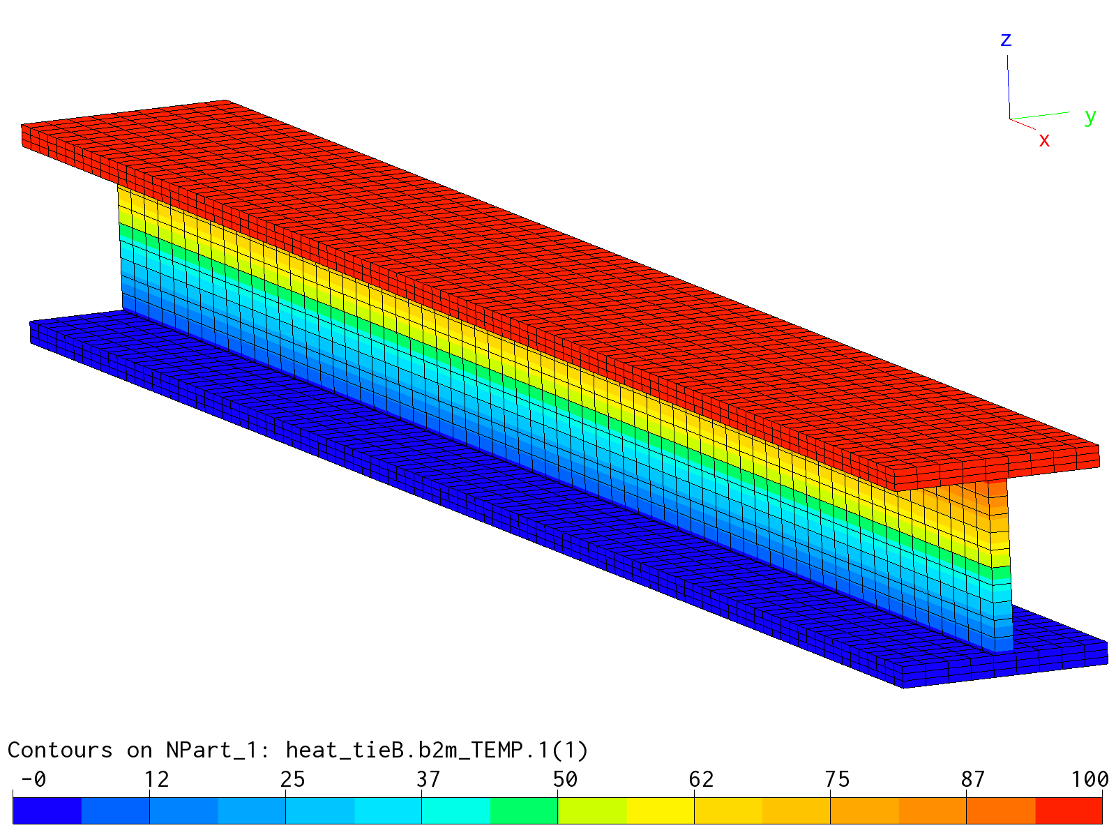
Heat analysis solution (temperatures) of mesh B.
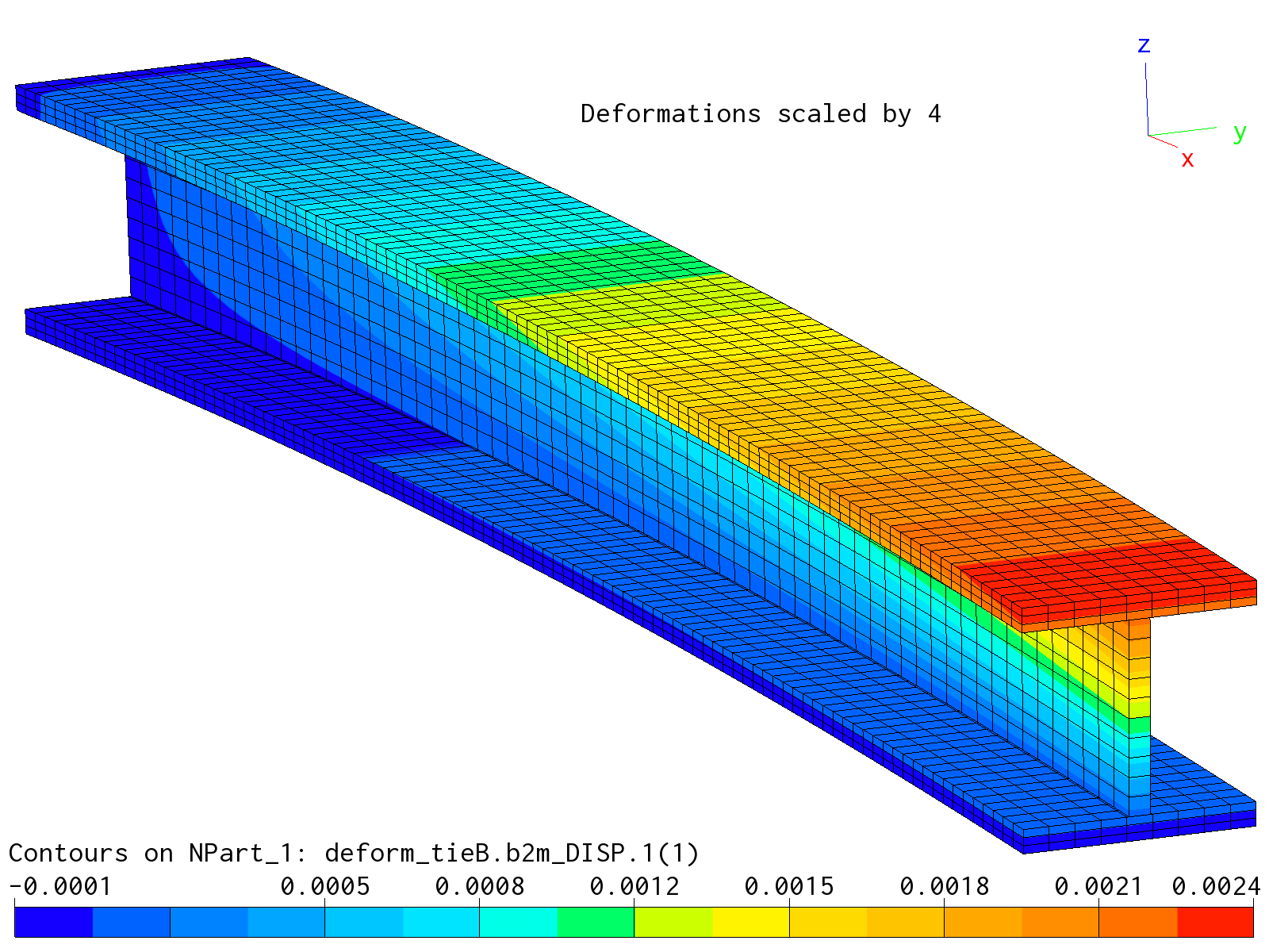
Deformation solution condition C1 rof mesh B.
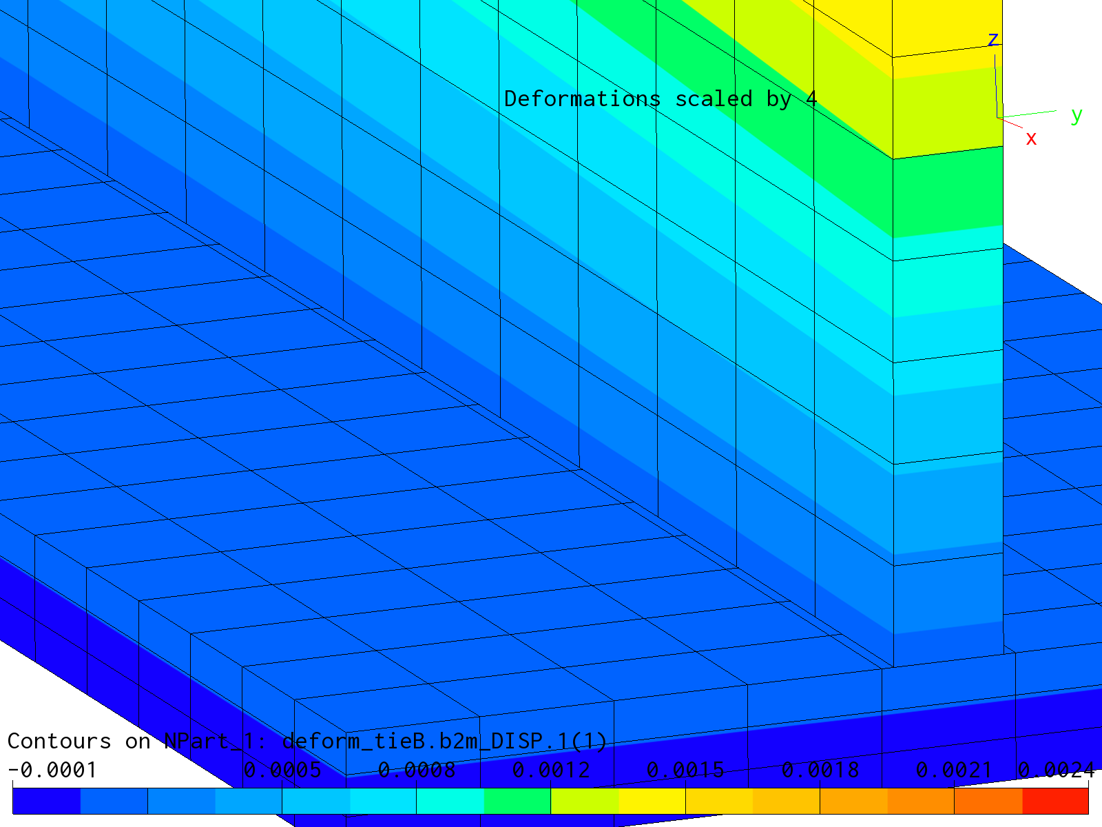
Deformation solution condition C1 for mesh B details showing detail of non-matching grid between flange and web.