5. Heat Transfer

5.1. Radiation of Plate to Plate

Location of test: $B2EXAMPLES/heat_flow/radiation_plate_plate

A plate steadily radiates heat on another plate with the same normal. This example demonstrates the radiation view factor capabilities of B2000++. An analytical solution is available for the view factor in the text book by Siegel and Howell [siegel].

Two rectangular plates are meshed independently one of the other as shown in the figure below. If only radiation elements (Q4 elements) are used, the solution will consist of exchanged heat between the hot plate (plate 1) and the cold plate (plate 2). Since all nodes of the hot plate (plate 1) have prescribed heat (essential boundary condition!) all nodes of plate 1 are constrained to the prescribed heat, and B2000++ has to solve for the non-linear essential boundary conditions imposed by the radiation.

Special attention has to be brought to the directions of the normals of the surfaces (see figure). If the normals are not oriented properly the structures will not radiate in the desired directions.

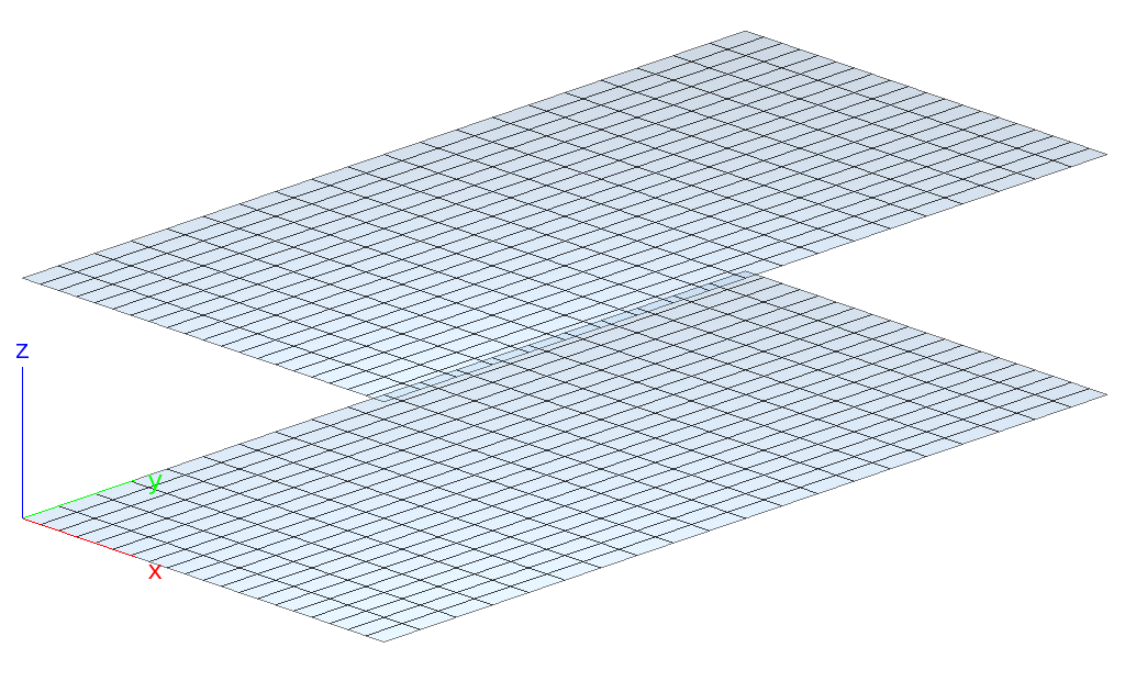
Radiation of plate to plate: Mesh and normals

Radiation problems are nonlinear as specified in the adir command below, and the nonlinear steady-state response is calculated with the default non-linear solver of B2000++, with the parameters defined in the case command (see input file radiation_plate_plate.mdl):

case 1
  ebc 1 # Heat on plate 1
  component radiation_heat NBC "VISI_RAD" # Radiation 1 to 2
  step_size_init 1
  step_size_min 1
  step_size_max 1
end

adir
   analysis nonlinear
   case 1
end

Observe the component radiation_heat NBC "VISI_RAD" instruction: It will generate the visibility matrix and exchange heat during the nonlinear solution process.

By setting the initial step size, the minimum step size, and the maximum step size to 1, the solver will try to solve the problem for the final step (default step is 1) with one step.

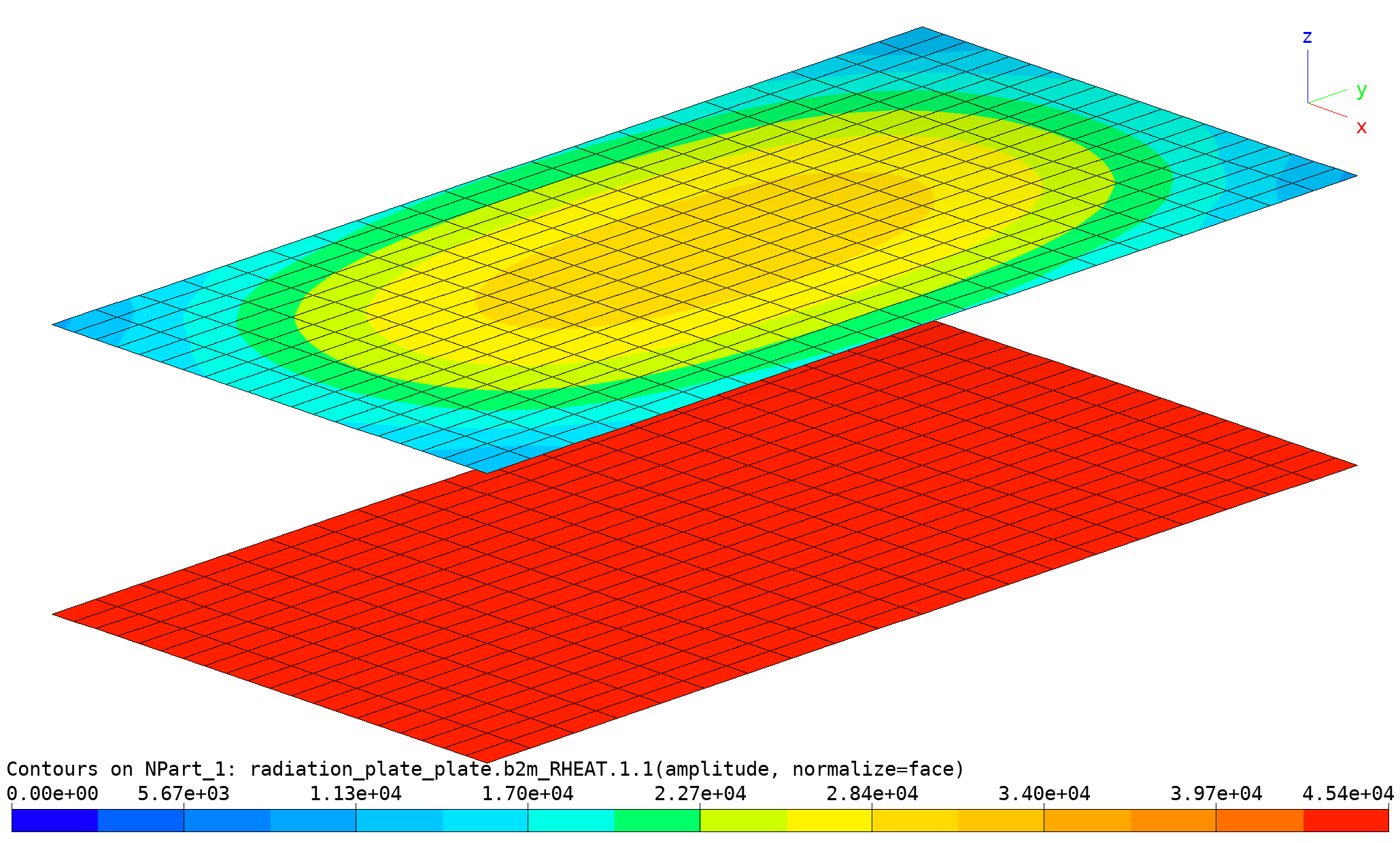
Radiation of plate to plate: Accumulated radiation heat. See script bv-view.py

The test procedure also computes the sum of heat accumulated in each plate (see test input file __init__.py):

model = si.Model('b2test.b2m') # Load model
last_step =  model.get_case(1).get_last_step()

# Load residual heat array
rheat = si.NodeField(model, 'RHEAT', case = 1, cycle = last_step)

nodes = model.get_epatch_body_node_set(1) # Get all nodes of patch 1
h1 = float(rheat.sum(rows=nodes)) # Sum up heat of all nodes involved

# Compute total heat received by plate 2

nodes = model.get_epatch_body_node_set(2) # Get all nodes of patch 2
h2 = float(rheat.sum(rows=nodes)) # Sum up heat of all nodes involved

a = 1.0
b = 2.0
h1_theor = 0.8 * 5.67e-8 * 1000**4 * a*b # Total heat of plate 1

# Compute view factor F12
# (how much of plate 1 heat is transferred to plate 2?)
c = 0.5
X = a / c
Y = b / c
F12 = 2 / (math.pi * X * Y) * (
    math.log(((1 + X**2) * (1 + Y**2) / (1 + X**2 + Y**2))**(1 / 2.0))
    + X * math.sqrt(1 + Y**2) * math.atan(X / math.sqrt(1 + Y**2))
    + Y * math.sqrt(1 + X**2) * math.atan(Y / math.sqrt(1 + X**2))
    - X * math.atan(X) - Y * math.atan(Y))

By setting TEST = 1 in __init__.py the test procedure prints the results:

b2testrunner .

Total heat of plate 1 (sum of  heat at nodes) h1 = 90720
Total heat of plate 2 (sum of  heat at nodes) h2 = -46175
Analytically computed view factor F12 = 0.50899
Total analytically computed heat of plate 1 = 90720
Total analytically computed heat of plate 1 = h1*F12 = 46175
Difference to analytically computed heat = 0.000%

The approximate analytical value for the radiation configuration factor based on pure geometric considerations can be found in the text book by Siegel and Howell.

5.2. Transient Heat Conduction in Soil

Location of example case: $B2EXAMPLES/heat/soil_freezing

The cooling of soil under a constant temperature of the air in the atmosphere and an initial temperature of the soil is calculated for a period of 60 days, the example being taken from the text book by Kreith and Bohn [kreith]. This 3D example demonstrates the step size control of the non-stationary nonlinear heat analysis solver.

The soil is modeled by a row of solid heat conduction elements (HE8 elements) extending 3 m down in the soil (z-direction). The soil is assumed to be semi-infinite, thus, a row of elements is sufficient, with free faces in the x- and y-directions. The face of the model which is in contact with the atmosphere is permanently set to -15 °C, while the rest of the model is set +20 °C for t=0. It is assumed that the conduction properties of the soil are uniform and linear and no convection or radiation between the soil and the atmosphere are taken into account.

The FE mesh is generated with a single epatch, with the face f1 of the epatch being in contact with the air at \(x=0\) (see figure below).

Transient heat conduction in Soil: Mesh and boundary conditions.

The essential boundary conditions are a temperature of -15 °C on the face which is exposed to the air:

ebc 1
  value -15. dof 1 epatch 1 f1
end

The initial conditions at the mesh nodes specified by means of the dof_init command:

dof_init 1
  value 20 allnodes      # Initially all nodes
  allow_override yes     # Default is 'no'
  value -15. epatch 1 f1 # Overwrite nodes of face to air to match ebc
end

The transient response is calculated with the nonlinear transient solver, and the solution is controlled by the case and stage commands.

By default the solver increments the time parameter from 0.0 to 1.0. In this example the time parameter range is from 0 to 60 days, i.e. 5184000 seconds. The best way of specifying this range is by introducing a case with a stage and by scaling the stage with the time_step option:

case 1
  analysis              dynamic_nonlinear # Although problem is linear
  stage 2 time_step     5184000   # Time is (60 days in seconds)
end

The stage 2 (see listing below) then defines the parameters of the actual case to be computed: The initial conditions and the essential boundary conditions, no natural boundary conditions being defined in this model.

The essential boundary conditions are activated with the ebc option of case 2:

ebc 1 sfunction '1'

By default, non-zero essential and natural boundary conditions are scaled by the analysis time. Specifying sfunction 1 tells the solver to keep the ebc constant in time.

By default, the nonlinear transient uses its error estimator to determine the step size, which results in a good computational efficiency. The option tol_dynamic sets the normalized maximum time integration error. Setting this to a lower value will increase accuracy but will result in a larger number of time steps. Conversely, setting this to a higher value will result in a faster analysis at the expense of accuracy.

stage 2
  dof_init       1               # Initial conditions
  ebc            1 sfunction '1' # Keeps ebcs constant
  tol_dynamic    0.01            # Time integration error control
end

Finally, the adir command specifies the analysis case to be solved:

adir
  case 1
end

The temperature at a given mesh node (at 0.7 m below the surface) as a function of time for several runs with a different dynamic error tolerance is executed with a Simples script (see file run.py):

# Run B2000++ with several time integration error tolerances TOLD,
# extract solutions, and add to list 'solutions' for plotting.

solutions = []
for told in (1000., 1., 0.1):
    os.system('b2000++ -define TOLD=%g soil.mdl' % told)
    model = si.Model('soil.b2m')
    x = model.get_steps(key = 'TIME')
    y = model.get_dof_value_of_steps('temperatures', 8, 1)
    model.close()
    solutions.append((x, y, told))

The solution list is then taken up by the graph generation section of run.py, which generates a PNG file:

plotted in the figure below. The dynamic error tolerance controls the time step: When the dynamic error tolerance is high (red markers in the graph below), less steps are performed, at the expense of accuracy. Note that the graph below is created with the Simples tools (see run.py script).

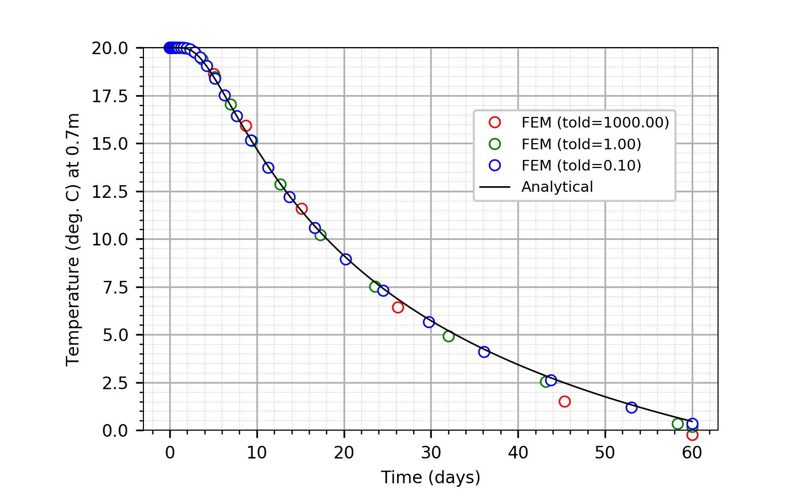
Transient Heat Conduction in Soil: Temperature T(t) at z=0.7[m]. The dynamic error tolerance controls the time step: When the dynamic error tolerance is high (red markers), less steps are performed, at the expense of accuracy.

Note: A constant step size - at the expense of accuracy - can be achieved by setting the step_size_init, step_size_max, and step_size_min options to the same fixed value, and by specifying a high tolerance for the time integration error with the tol_dynamic option:

stage 2
  step_size_init 86400           # 1 day
  step_size_max  86400           # Keeps step size constant
  step_size_min  86400           # Keeps step size constant
  tol_dynamic    10000           # Time integration error control
  dof_init       1               # Initial conditions
  ebc            1 sfunction '1' # Keeps ebcs constant
end

The analytical function can be found in the textbook by Kreith and Bohn [kreith] and it is programmed in the run.py script.