4. Dynamic Problems

4.1. Cable-Stayed Bridge

Location of example: $B2EXAMPLES/dynamic/bridge

The lowest eigenfrequencies and their corresponding eigenmodes of a cable-stayed steel-concrete composite bridge are calculated. A global FE model of the structure, with shell and beam elements, has been established. Although the problem of cable-stayed structures is geometrically non-linear it is approximated here by replacing the cable by beams with a given prestress.

The FE model of the Zaltbommel bridge in the Netherlands has been elaborated by the NLR, the mesh consisting of R.S rods, B2.S.RS beams, and Q4.S.MITC quad shell elements. The rod and beam elements refer to steel, whereas the shell elements refer to concrete.

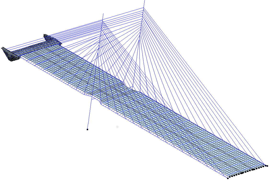
FE mesh.

The free vibration analysis with B2000++ is controlled with the MDL commands adir and case, requesting the 20 lowest eigenfrequencies:

case 1
  analysis free_vibration
  nmodes 20
  ebc 1
end

adir
  case 1
end

The cases option of adir specifies which cases B2000++ should process (here: process case 1). In its turn, the case 1 description in the cases command specifies the analysis type and other options related to that particular type of analysis:

• The analysis option of case indicates the type of analysis to be performed. free_vibration will launch the B2000++ free vibration analysis solver (see also comment below).

• The nmodes option specifies the number of eigenmodes or eigenvalues to be computed. In the absence of a shift the smallest nmodes eigenvalues around 0.0 are computed.

By default B2000++ calculates the real symmetric eigenvalue problem with the Implicitly Restarted Lanczos Iteration variant of the Implicitly Restarted Arnoldi Iteration algorithm implemented in the ARPACK, the ARnoldi PACKage library. In addition, the model mass and modal stiffness for each mode are computed. Results are summarized below, printed with the print_eigenfrequencies.py script. Alternatively, results can be displayed with the b2browser application.

prompt> b2print_eigenfrequencies zaltbommel

Free vibration eigenfrequencies, case=1, cycle=0
Spectral shift=0, where="SM (around the shift value)", Termination=NORMAL

 Mode       lambda        Omega    Frequency      Modal_K      Modal_M
 1        7.216        2.686       0.4275        7.216            1
 2        7.634        2.763       0.4397        7.634            1
 3         16.2        4.025       0.6407         16.2            1
 4        19.13        4.374       0.6961        19.13            1
 5         19.4        4.404        0.701         19.4            1
 6        27.51        5.245       0.8348        27.51            1
 7        36.23        6.019       0.9579        36.23            1
 8        53.11        7.288         1.16        53.11            1
 9        58.47        7.647        1.217        58.47            1
10           61         7.81        1.243           61            1

Results can be rendered directly with the baspl++ viewer. Eigenmodes are visualized either with baspl++’s built-in modes viewing tool. The viewer script view.py produces the plot shown below:

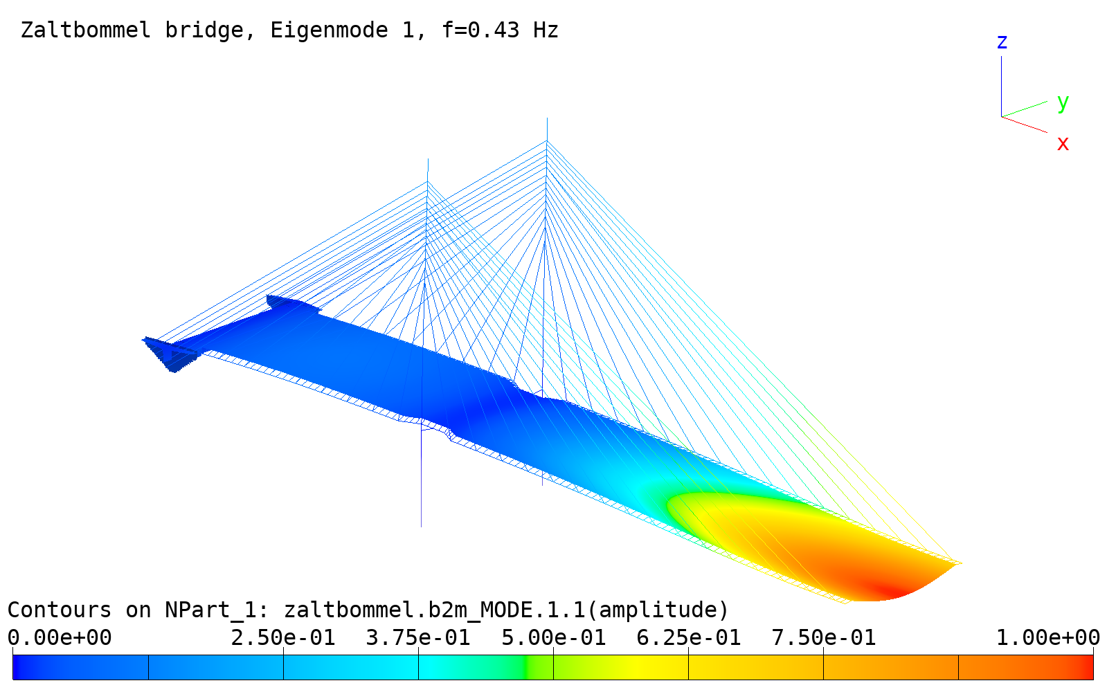
First fundamental free vibration mode no. 1.

Any other mode i can be rendered with the baspl++ function mode (see below):

mode(i)

view.py also provides a function for producing plots of several modes:

def mode(imode):
    """Render mode 'imode' (int).
    """
    m2.field.ch.mode = imode
    f = m.db["MODE.1.0.0.1.{}".format(imode)].desc["FREQ"][0]
    s.label = 'Zaltbommel bridge, Eigenmode {}, f={:.2f} Hz'.format(imode, f)

def images(i,j):
    """Render modes from `i` to `j` in ``png`` files.
    """
    for k in range(i, j+1):
        mode(k)
        s.export_to_file("mode{:03d}.png".format(k))

Calling the above defined function

images(1,8)

from the baspl++ shell will render modes 1 to and produce 8 png files mode001.png to mode008.png that can be assembled to one single plot with the montage application:

montage *.png -scale 33% -mode Concatenate -tile 2x8 montage.png

producing

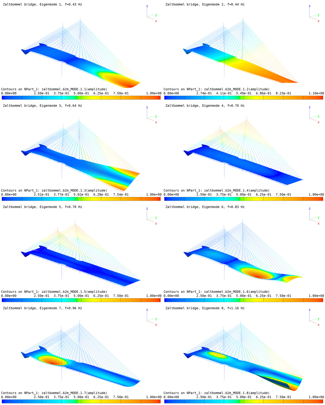
Modes 1 to 8 assembled in one single plot with the montage application.

4.2. One-DOF Oscillator

Location of example: $B2EXAMPLES/dynamic/one_dof_oscillator

This transient test case is the simplest possible test - a one-DOF oscillator. The test case checks the response over a time interval for applied initial displacement, applied initial velocity, force consatnt over time, and sinusoidal force over time.

The oscillator is modeled with a single rod element of length \(L\), cross section area \(A\), and modulus of elasticity \(E\). Node 1 of the rod is fixed, and node 2 moves in x-direction. The mesh, the material, and the constraints are defined in MDL file r2.mdl:

nodes
  1 0. 0. 0.
  2 (L) 0. 0.
end

elements
  type R2.S
  mid 1
  area (A)
  1 1 2
  type PMASS3.S
  mass (MASS)
  100 2
end

material 1
  type isotropic e (E) p 0.0 density 0.0
end

ebc 1 # Constraints (zero value boundary conditions)
  value 0. dof 1/3 nodes 1 dof 2/3 nodes 2
end

Test are performed with the dynamic nonlinear solver, because the dynamic linear solver is too restrictive (see comment). Since displacements are very small the solution will be very close to the linear analytical solution.

All cases define the same MDL case block:

case 1
   analysis dynamic_nonlinear
   tol_dynamic 1e10 # = no time integration error control
   stage 11 sfactor (T) # Here we go from time=0.0 to time=T
end

4.2.1. Initial Displacement

Specifying an initial displacement at time=0.0 will create an oscillation with an amplitude equal to the initial displacement. initial_displacement.mdl formulates the case (see comments), with the initial condition defined as

# Initial condition to be included in analysis at time=0.0, i.e for
# the first stage. Assign initial displacement to DOF 1 of node 2.
dof_init 123
  value (DOF_INIT) dof 1 node 2
end

and the corresponding stage (see case block above) defining the initial displacement set:

stage 11
   ebc 1
   dof_init 123 # Initial condition at time=0.0
   step_size_init (DT) # Must be defined if sfactor != 1.0
   step_size_min (0.01*DT) # Must be defined if sfactor != 1.0
   step_size_max (DT) # Must be defined if sfactor != 1.0
end

The case is launched with the Python script test_initial_displacment.py which produces the plot file initial_displacement.png:

python3 initial_displacement.py

Displacement and velocity diagrams for the oscillator are generated with the plot function of util.py.

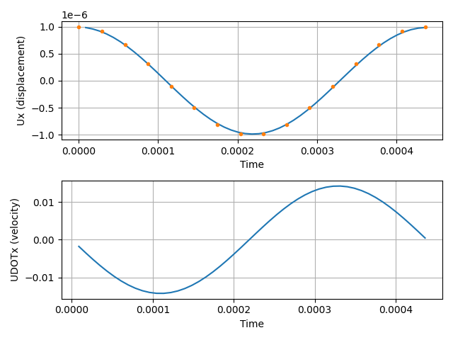
Displacement and velocity diagrams (orange: analytical solution).

4.2.2. Initial Velocity

Specifying an initial velocity at time=0.0 will induce a sinusoidal oscillation. initial_velocity.mdl formulates the case, with the initial condition defined as

# Initial time-derivative condition to be included in analysis at
# time=0.0, i.e for the first stage. Assign initial velocity
# to DOF 1 of node 2.
dofdot_init 123
   value (UDOT0)
   node 2
end

and the corresponding stage defining the initial velocity set:

stage 11
   ebc 1
   dofd_init 123 # Initial time-derivative  condition at time=0.0
   step_size_init (DT) # Must be defined if sfactor != 1.0
   step_size_min (0.01*DT) # Must be defined if sfactor != 1.0
   step_size_max (DT) # Must be defined if sfactor != 1.0
end

The case is launched with the Python script test_initial_velocity.py which produces the plot file initial_velocity.png:

python3 initial_velocity.py

Displacement and velocity diagrams for the oscillator are generated with the plot function of util.py.

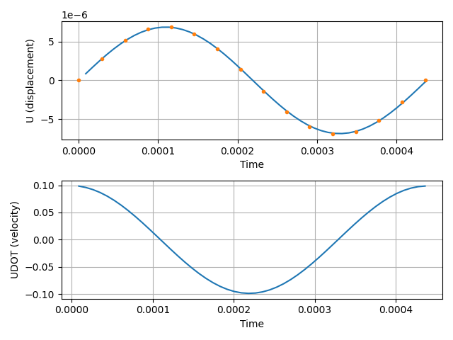
Displacement and velocity diagrams (orange: analytical solution).

4.2.3. Constant (Step) Force

A constant force \({F_x}\) defined in nbc set 1 (see r2.mdl) is applied to node 2. The force is constant over the time interval. The corresponding stage specifies the (constant) sfunction as 1, see constant_force.mdl):

stage 11
   ebc 1
   nbc 1 sfunction '1'
   step_size_init (DT) # Must be defined if sfactor != 1.0
   step_size_min (0.01*DT) # Must be defined if sfactor != 1.0
   step_size_max (DT) # Must be defined if sfactor != 1.0
end

The case is launched with the Python script test_constant_force.py which produces the plot file constant_force.png:

python3 constant_force.py

Displacement and velocity diagrams for the oscillator are generated with the plot function of util.py.

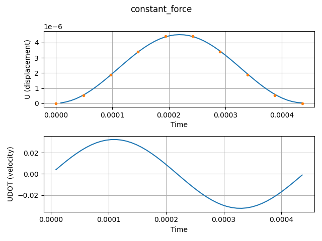
Displacement and velocity diagrams (orange: analytical solution).

4.2.4. Forced Vibration

A sinusoidal force \(F_x=\sin{\overline{\omega} t}\), with \(\overline{\omega}=0.667\omega\) and circular frequency \(\omega=\frac{AE}{L}\), is applied to node 2. The corresponding stage specifies the sfunction as sin(9601.1*t), see forced_vibration.mdl):

stage 11
   ebc 1
   nbc 1 sfunction 'sin(9601.1*t)'
   step_size_init (DT) # Must be defined if sfactor != 1.0
   step_size_min (0.01*DT) # Must be defined if sfactor != 1.0
   step_size_max (DT) # Must be defined if sfactor != 1.0
end

The case is launched with the Python script test_forced_vibration.py which produces the plot file forced_vibration.png:

python3 forced_vibration.py

Displacement and velocity diagrams for the oscillator are generated with the plot function of util.py.

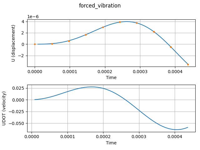
Displacement and velocity diagrams (orange: analytical solution).

4.3. Linear Transient Analysis of Beam

Location of example: $B2EXAMPLES/dynamic/simple_beam

A simply supported beam is loaded by a central load P applied at time t=0 (see also input file beam.mdl). The model has been chosen such that the response under the given loads is linear and the beam thickness to beam length ratio is small, thus rendering the influence of the shear strain negligible. A theoretical transient solution for this configuration is available, formulated with the Euler beam theory [clough]:

\[Dy(t) = \frac{P_{0}L^{3}}{n^{4}EI} \sum_{n=1,3,5} \frac{1 - \cos(\omega_{i}t)}{i^4}\]

where i is the odd (symmetric around \(y = L/2\)) mode number, E the modulus of elasticity, I the moment of inertia around the bending axis, m the beam mass per length unit, and L the length of the beam, and \(Ft(t) = P_0\).

The force is applied at \(t=0\) and kept constant. The beam as displayed below is modeled with B2.S.RS beam elements, see MDL input file beam.mdl.

Beam model.

Three different analyses will be carried out: A static analysis, a free-vibration analysis, and a transient analysis. Hence, three different analysis cases will be defined. All three cases refer to the same essential boundary conditions (MDL)

ebc 1
  # Eliminate dof's 3,4,5
  value 0.0 dof [UZ RX RY] allnodes
  # Support
  value 0.0 dof [UX UY] epatch 1 P1 dof 2 epatch 1 P2
end

Natural boundary conditions will be applied to the static and transient dynamic analysis:

nbc 1
  value 1000. dof UY node 21
end

The static analysis case 1 includes both the essential and the natural boundary conditions defined above:

case 1
  analysis linear
  nbc 1
  ebc 1
end

A free vibration analysis gives an idea about the frequencies to be expected, at the same time checking the free vibration analysis solution and preparing the input for the modal analysis (see the text book by Clough and Penzien [clough]). Theoretical free vibration modes and their corresponding circular frequencies \(\omega\) are available with

\[\omega_{i} = i^{2}\pi^{2}\frac{\sqrt{EI}}{mL^{4}}\]

The free vibration analysis case is defined by specifying the essential boundary condition set and the number of (lowest) eigenvalues to be computed:

case 2
  analysis free_vibration
  nmodes 10
  ebc 1
end

The free vibration analysis solution is obtained by explicitly requiring case 2 in the adir command:

adir
  case 2
end

Eigenvalues are obtained by executing b2000++ and by printing them with the Simples print_eigenfrequencies.py script:

$ b2print_eigenfrequencies --case=2 beam

Eigenfrequencies, case 2
Mode    Frequency        Omega      Modal_K      Modal_M
   1         10.5        65.96        625.2     2.72e+06
   2        41.81        262.7        404.6    2.792e+07
   3        93.42          587        184.7    6.363e+07
   4        144.9        910.6        624.8    5.181e+08
   5        164.5         1034        107.7     1.15e+08
   6        254.1         1597        71.99    1.835e+08
   7        361.1         2269        52.58    2.706e+08
   8          435         2733        623.6    4.658e+09
   9        484.2         3043        40.84     3.78e+08
  10        622.6         3912        33.19    5.078e+08

Note that the theoretical circular eigenfrequencies are derived from an Euler beam model. Thus, the shear, which has a certain influence for the present model (although the beam is slender), is not taken into account and explains small differences between theoretical and calculated circular eigenfrequencies.

While the modal solver takes the damping coefficients of each mode \(\zeta\) for the model from the argument list, the transient solver requires the Rayleigh damping coefficients (see [bathe1996] \(\alpha\) and \(\beta\) to be defined:

\[\alpha = \frac{2 \omega_1 \omega_2 (\omega_1 \zeta_2 - \omega_2 \zeta_1)} {\omega_{1}^{2} - \omega_{2}^{2}}\]

\[\beta = \frac{2(\omega_1 \zeta_1 - \omega_2 \zeta_2)}{\omega_{1}^{2} - \omega_{2}^{2}}\]

\(\omega\) and \(\zeta\) are the circular frequencies and the damping percentage, respectively.

The B2000++ transient solver and the modal analysis script msolve are executed without damping or with 10% damping, see the Makefile in the examples directory. The damped transient analysis eventually converges to the static solution, given a damping coefficient >0. The modal analysis test selects the first 3 eigenvalues.

With circular frequencies available from the free vibration analysis, the modal transient analysis can be performed, either with the b2modal program or with the python script msolve (see example directory):

./msolve ${NELEM} ${MIDSTATION} ${T1} ${NSTEPS} 0.0

msolve calls the Simples Modal Transient Solver.

The time response curve for the beam mid-station y displacement Uy (10% damped response) is obtained with the Simples script plot_time_history (see Makefile in the example directory). It produces the svg file dy.svg:

Modal transient analysis: Time-displacement response, no damping.

Modal transient analysis: Time-displacement response, 10% damping.

A linear transient analysis without damping or with Rayleigh damping is defined in case3, which is split in the effective case definition (case 3) and the stage definition (case 31). Adding a stage is necessary for specifying the time range (time_step):

case 3
  title 'Transient analysis'
  stage 31 time_step (T)
end

stage 31 integrates from time 0.0 to T, T being a parametrized value (see file beam.mdl).

The stage in its turn defines conditions of the stage:

stage 31
  nbc 1 sfunction '1.'
  ebc 1
  step_size (DT)
end

nbc 1 sfunction '1.'includes the nbc set 1, scaling it to 1.0 for the whole stage. ebc 1 includes the nbc set 1, keeping it constant during the stage (default). multistep_integration_order selects the time integration scheme, here of order 2. step_size defines the time step or increment, (DT) being a parametrized value.

The transient analysis solution is obtained by explicitly requiring case 3 in the adir command:

adir
  case 3
end

Direct transient analysis: Time-displacement response, no damping.

Direct transient analysis: Time-displacement response, 10% Rayleigh damping.

The shell command

make all

executes all damped/non-damped tests with the direct transient and the modal solvers and produces csv files. These can then be combined to comparison plots. Example:

b2plot_csv --l=center --width=150. --height=50. modal_0.0.csv transient.csv

produces the comparison plot

Compare linear modal and transient curves, mid-station DY displacement, no damping.

and

b2plot_csv --l=center --width=150. --height=50. modal_0.1.csv transient_10.csv

produces the comparison plot

Compare linear modal and transient curves, mid-station DY displacement, 10% damping.

4.4. Free Vibration of Unconstrained Beam

Location of example: $B2EXAMPLES/dynamic/unconstrained_vibration

The lowest eigenfrequencies of an unconstrained straight beam are computed. When one tries to solve the eigenvalue problem \(K x = \lambda M x\) of an unconstrained structure the procedure usually fails, unless a spectral shift \(\sigma\) is applied:

\[K x = (\lambda - \sigma) M x\]

The straight slender beam is 100cm long and has a solid rectangular cross section of width=0.3cm by height=1cm. Material is aluminum. Units are formulated in the MKS system.

Tests are performed with B2.S.RS and B3.S.RS beam elements. As expected the eigenvalue analysis procedure fails without a spectral shift. However, with a small shift the procedure works. The run with B2.S.RS elements produces the following 10 first eigenvalues:

Free vibration eigenfrequencies, case=1, cycle=0
Spectral shift=1, where="SM (around the shift value)", Termination=NORMAL

Mode       lambda        Omega    Frequency      Modal_K      Modal_M
   1 -4.99227e-05            0            0            0            0
   2 -1.95039e-05            0            0            0            0
   3 -1.60658e-05            0            0            0            0
   4 -1.41603e-05            0            0            0            0
   5 -1.25672e-05            0            0            0            0
   6 -1.14704e-05            0            0            0            0
   7      9860.68      99.3009      15.8042  0.000964875      9.51432
   8      74981.7      273.828      43.5811   0.00033697      25.2666
   9       109497      330.904       52.665   0.00096561      105.732
  10       288504      537.126      85.4862  0.000171843      49.5775

Note that the first 6 eigenmodes are rigid body modes (negative eigenvalues \(\lambda\)) and they are the only ones found to the left of the shift. Mode 7 and 9 (see figure below) are the first fundamental modes around the z-axis and the y-axis. The eigenfrequencies agree well with the theoretical values obtained from [Roark] (table 16.1, uniform beam, both ends free).

\[c \sqrt{\frac{E I} {m L^4}}\]

where \(c=22.4\) for the first fundamental mode.

Eigenfrequencies comparison [Hz]. B2.S.RS beam elements.

Mode	B200++	Analytical
7 (bending around global z-axis)	15.80	15.821
9 (bending around global y-axis)	52.67	52.737

The baspl++ script view.py produces plots (png files) of the first 10 eigenmodes.

baspl++ -t view.py beam.b2m

The plots can be merged into on single png file montage.png with the Linux montage program:

montage mode*.png -scale 33% -mode Concatenate -tile 2x5 montage.png

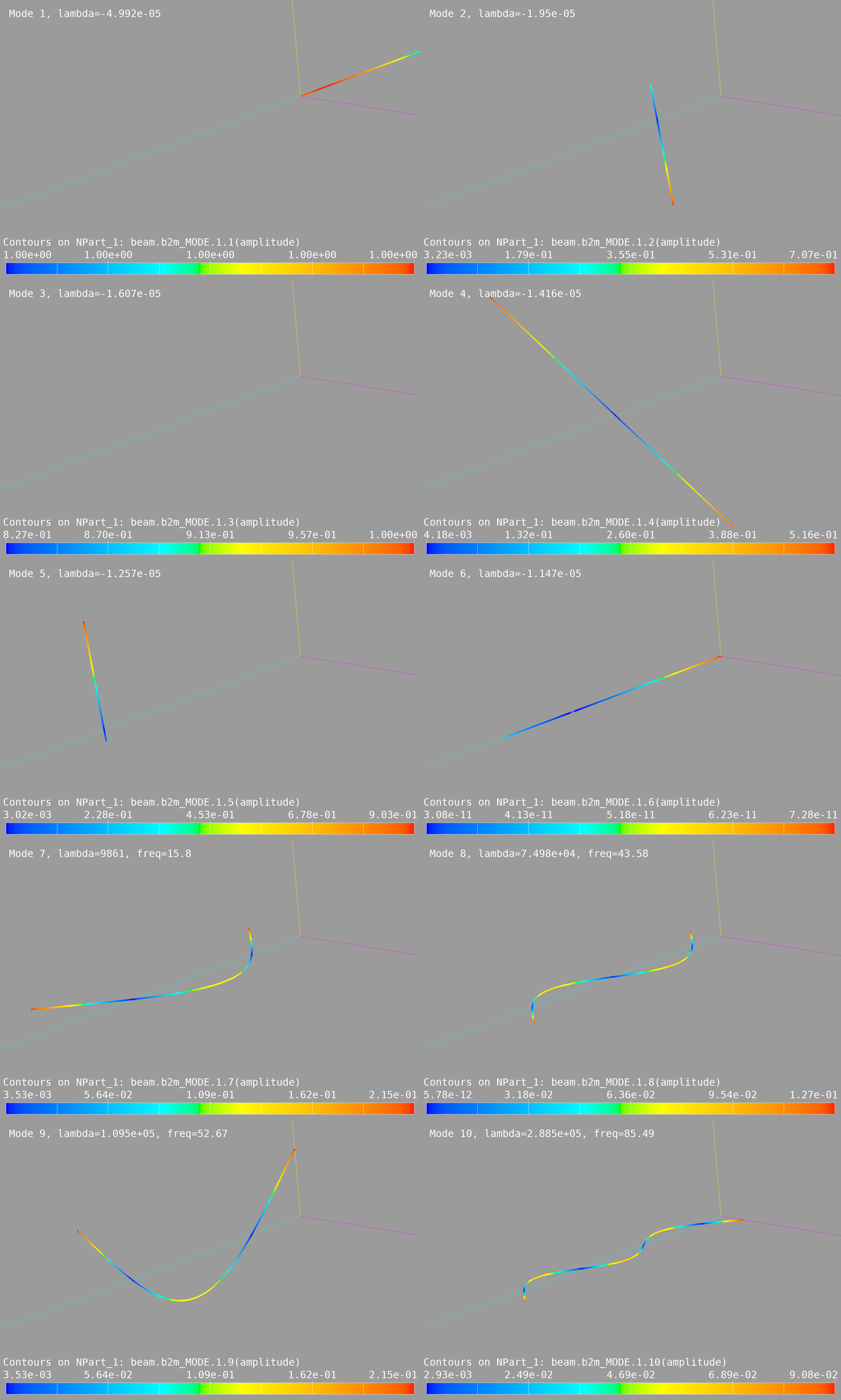
Unconstrained beam: First 10 eigenmodes.